Wheel speed estimation using a drivetrain model

Description

BACKGROUND

The invention relates to systems and methods for determining the speed of a driven wheel. Specifically, the invention determines the speed of a driven wheel using the speed of a drive shaft and the speed of a second driven wheel, and compensates for timing factors.

Vehicle systems, such as electronic stability control systems, require knowledge of the speed of each of the wheels of the vehicle. The speed of the wheels needs to be accurately determined in near real time (e.g., every 5 milliseconds). To achieve this, many modern vehicles use wheel speed sensors on each wheel with the sensors hard-wired to the control system or linked via a communication bus.

SUMMARY

In one embodiment, the invention provides a controller. The controller includes a processor and a non-transitory computer readable medium. The processor is configured to receive the speed of a first driven wheel from a wheel speed sensor and the speed of a drive shaft from a drive shaft sensor. The non-transistory computer readable medium includes program instructions executed by the processor for determining a speed of a second driven wheel based on a plurality of detected speeds of the first driven wheel and detected speeds of the drive shaft over time.

In another embodiment the invention provides a method of determining a speed of a first wheel of a vehicle. The vehicle includes a controller, a differential, a second driven wheel, and a drive shaft. The first and second wheels are driven by the drive shaft. The method includes detecting a speed of the second driven wheel, the second driven wheel driven by the differential, detecting a speed of the drive shaft, the drive shaft driving the differential, transmitting the speed of the second driven wheel to the controller, transmitting the speed of the drive shaft to the controller, compensating for delays in transmission of the speed of the second driven wheel and the drive shaft, compensating for differences in when the speed of the second driven wheel is detected and when the speed of the drive shaft is detected, and determining a speed of the first wheel, using the speed of the second driven wheel, the speed of the drive shaft, and the compensating acts, the first wheel driven by the differential.

Other aspects of the invention will become apparent by consideration of the detailed description and accompanying drawings.

BRIEF DESCRIPTION OF THE DRAWINGS

FIG. 1 is a block diagram of a vehicle.

FIG. 2 is a chart showing an actual wheel speed and communication and computation delays.

FIG. 3 is a chart showing the impact of different update intervals for a plurality of speed sensors on a calculation of a wheel speed.

FIGS. 4A and 4B are a schematic of an acceleration model for determining a wheel speed.

FIG. 5 is an exploded view of an open differential showing various torque transfer values.

DETAILED DESCRIPTION

Before any embodiments of the invention are explained in detail, it is to be understood that the invention is not limited in its application to the details of construction and the arrangement of components set forth in the following description or illustrated in the following drawings. The invention is capable of other embodiments and of being practiced or of being carried out in various ways.

FIG. 1 shows a block diagram of a vehicle 100. The vehicle 100 includes a right front wheel 105, a left front wheel 110, a right rear wheel 115, a left rear wheel 120, an engine 125, a transmission 130, a drive shaft 135, a drive shaft sensor 140, a differential 145, a right rear axle 150, a left rear axle 155, a right front wheel speed sensor 160, a left front wheel speed sensor 165, and a right rear wheel speed sensor 170. The vehicle 100 also includes a controller 175 (e.g., an electronic stability controller (ESC)) and a communication network 180 (e.g., a controller area network (CAN) bus). In some embodiments, the controller 175 and/or other modules include a processor (e.g., a microprocessor, microcontroller, ASIC, DSP, etc.) and memory (e.g., flash, ROM, RAM, EEPROM, etc.; i.e., a non-transitory computer readable medium), which can be internal to the processor, external to the processor, or both. The processor executes program code stored in the memory. Portions of the invention can be implemented in hardware or software or a combination of both.

The wheel speed sensors 160, 165, and 170 detect the speed of their respective wheels and communicate that speed to the controller 175. The speed can be communicated via the communication network 180 or directly (e.g., an analog signal, a PWM signal, etc.). Similarly, the drive shaft speed sensor 140 detects the speed of the drive shaft 135 and communicates that speed to the controller 175. The differential 145 is driven by the drive shaft 135 and divides the torque between the left and right rear wheels 120 and 115 such that the wheels can turn at different rates. The sum of the speeds of the left and right rear wheels 120 and 115 is two times the speed of the drive shaft 135 (assuming a one to one gear ratio). The controller 175 estimates the speed of one of the driven wheels 115 and 120 as described below (for the description below, the controller 175 estimates the speed of the left rear wheel 120).

The speed of the left rear wheel 120 can be approximated using equation 1 below. Solving for L, the determined speed of the left rear wheel, provides equation 2 below:

T=(L+R)/2  (eq. 1)

L=2T−R  (eq. 2)

• • where T is the measured speed of the drive shaft 135, and R is the measured speed of the right rear wheel 115.

Determining the speed of the left rear wheel 120 using these equations is generally accurate enough for use with anti-lock braking systems which update approximately every 50 msec. However, an ESC system updates approximately every 5 msec. If the measured speeds of the right rear wheel 115 and/or the drive shaft 135 are communicated to the controller 175 via a communications network 180, the controller 175 receives the measured speeds after a delay exceeding the ESC update time. For example, FIG. 2 shows delays that were measured in a system using a CAN bus. The CAN bus had a worst case delay in providing the speed information to the controller 175 of 15 msec. In addition, the controller 175 requires time to process the data it receives. In this case, up to an additional 11 msec. The total delay reached 26 msec. A delay of 26 msec is more than five times the update time for the ESC system.

The error between actual speed of a wheel and the calculated wheel speed (e.g., due to the delays above) can be further exacerbated by differences in the update speeds of the different sensors. For example, FIG. 3 shows the deviation of the calculated speed of a left rear wheel 120 where the right rear wheel speed sensor updates every 5 msec and the drive shaft speed sensor 140 updates every 7 msec.

To improve the performance of the system, more accurate determination of the wheel speed is needed. By taking into account past conditions (versus using only the latest readings), models can be developed to accurately estimate wheel speed.

For an open differential, the speed of a driven left wheel is defined by

L(k)=2T(k)−R(k)

where:

• • k is the control loop cycle,
  • L(k) is the calculated speed of the left driven wheel at cycle k,
  • T(k) is the measured transmission output speed at cycle k, and
  • R(k) is the measured speed of the right driven wheel at cycle k.

Considering errors along with delays in the inputs for T and R, L(k) becomes L(k)=F(T(k), T(k−1) . . . R(k), R(k−1) . . . L(k), L(k−1) . . . other vehicle states) where:

• • F is a function of a plurality of input variables.

The invention uses models to estimate the function F. Three methods or models are used: acceleration, Taylor Series, and drivetrain modeling. The acceleration method uses the acceleration of the left driven wheel to estimate the speed of the left driven wheel at cycle k. The following equation is used to perform the estimation:

L(k)=L(k−1)+L′(k−1)(dt)

where:

• • L′ is the first derivative of L, and
  • dt is the cycle time.

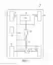
The calculations can be smoothed using a weighted average of several past cycles or a filtered value. Empirical vehicle data can also be used to limit a change in the estimated speed of the wheel to an absolute change. Acceleration can also be modeled as discussed below in relation to a drivetrain model. FIGS. 4A and 4B show a schematic of an acceleration model 100. A sensed speed of a right wheel 105 and a sensed speed of a driveshaft 110 are input into the model. As discussed above, the wheel speed sensor xxx and the driveshaft speed sensor xxx update their outputs at different time intervals (e.g., 5 msec for the wheel speed sensor xxx and 7 msec for the driveshaft speed sensor xxx). By using various multipliers 115, adder/subtractors 120, and delays 125, the model 100 is able to compensate for the differences in signal updates. A switch 130 connects a correct signal to an output 135. The model 100 includes a three additional outputs 140, 145, and 150 for testing purposes.

A Taylor Series is a representation of a function as an infinite sum of terms calculated from the values of its derivatives at a single point. A Taylor Series for modeling the speed of a left driven wheel takes the form:

L(k)=L(k−1)+L′(k−1)(dt)/1!+L″(k−1)(dt)²/2!

where:

• • L′ and L″ are derivatives of L, and
  • dt is the cycle time.

Again, the calculations can be smoothed using a weighted average of several past cycles or a filtered value. Empirical vehicle data can also be used to limit a change in the estimated speed of the wheel to an absolute change.

L(k) can also be estimated using various vehicle states including applied brake torque, friction co-efficient, and load on a wheel among others. The vehicle states can be calculated using a drivetrain model.

An example drivetrain model includes models of the (1) engine and torque converter pump assembly, (2) torque converter turbine and transmission input shaft, (3) transmission output shaft and drive shaft, (4) ring gear of the open differential, (5) torque transfer from the engine to the differential, (6) drive axle torque, and (7) total drive dynamics.

An engine and torque converter pump assembly model calculates the available torque converter pump output using engine combustion torque. Neglecting the elastic and friction term, the equation of motion can be simplified as:

T_p=T_e−J_eω_e  (eq. 1)

where:

• • T_p is the torque output at the pump assembly,
  • T_e is the engine torque resulting from combustion,
  • J_e is the moment of inertia of the engine crankshaft, flywheel and torque converter pump assembly, and
  • ω_e is the angular acceleration of the engine crankshaft, flywheel and torque converter pump assembly. In the software, the engine acceleration can be calculated from the engine speed.

Note: elastic, friction, and damping are neglected in the equations.

A torque converter turbine and transmission input shaft model calculates the available torque at transmission input shaft using:

T_I=T_pƒ(1/v)−J_Iω_I  (eq. 2)

where:

• • T_I is the torque output at the transmission input shaft,
  • ω_I is the angular acceleration of the transmission input shaft,
  • v is the speed ratio for the automatic transmission and is defined as,
    • ω_I=ω_e/v (Note: The above relation is not true for the angular acceleration of the torque converter.),
  • G(1/v) is the torque converter multiplication factor as a function of 1/v, and
  • J_I is the moment of inertia of the turbine and transmission input shaft.

A transmission output shaft and drive shaft model calculates the available torque at drive shaft from:

T_d=T_IG_tj−J_dω_d  (eq. 3)

where:

• • T_d is the available torque at the drive shaft pinion gear,
  • G_tj is the transmission gear ratio at jth gear,
  • J_d is the moment of inertia of the drive shaft (include transmission output shaft and its gear set), and
  • ω_d is the angular acceleration of the transmission output shaft.

The angular acceleration has the following relation:

ω_d=ω_I/G_tj  (eq. 3a)

The ring gear of the open differential model calculates the available torque at open differential ring gear using:

T_rg=T_dG_A−J_rgω_rg  (eq. 4)

where:

• • T_rg is the available torque at the ring gear (also referred to as Cardan torque).
  • G_A is the axle ratio,
  • J_rg is the ring gear assembly moment of inertia, and
  • ω_rg is the angular acceleration of the ring gear (also referred to as Cardan acceleration).

The speed relation among ring gear, drive shaft and wheel speed is:

ω_rg=ω_d/G_A=(ω_AR+ω_AL)/2  (eq. 4a)

where:

• • ω_AR is right driven axle acceleration, and
  • ω_AL is left driven axle acceleration.

FIG. 5 shows the location of the torque transfer variables in an open differential.

A torque transfer from engine to differential model calculates the available torque at the ring gear. The available torque at the ring gear can be described by engine combustion torque, engine rotational acceleration, and wheel rotational acceleration (a known variable).

Substituting torque equations (1), (2) and (3) into equation (4), results in:

T_rg={[T_e−J_eω_e)ƒ(1/v)−J_Iω_I]G_tj−J_dω_d}G_A−J_rgω_rg  (eq. 5)

Substituting speed equation (3a) and (4a) into equation 5 and simplifying it results in:

T_rg=ƒ(1/v)G_tjG_AT_e−ƒ(1/v)G_tjG_AJ_eω_e−G_tj²G_A²J_I(ω_AR+ω_AL)/2−G_A²J_d(ω_AR+ω_AL)/2−J_rg(ω_AR+ω_AL)/2  (eq. 5a)

where:

• • ƒ(1/v)G_tjG_AT_e is the engine torque amplified by the torque converter, transmission, and axle,
  • ƒ(1/v)G_tjG_AJ_eω_e is the torque loss due to engine acceleration,
  • G_tj²G_A²J_I(ω_AR+ω_AL)/2 is the torque loss due to transmission input shaft acceleration,
  • G_A²J_d(ω_AR+ω_AL)/2 is the torque loss due to transmission output shaft acceleration, and
  • J_rg(ω_AR+ω_AL)/2 is the torque loss due to ring gear acceleration.

A drive axle torque model calculates the drive axle torque for each drive axle. For an open differential, each drive axle torque is approximately half of the ring gear torque when neglecting torque lost at the spider or similar gear.

T_AR˜T_rg/2˜_TRR_whl+T_bR+J_Aω_AR  (eq. 6)

T_AL˜T_rg/2˜F_TLR_whl+T_bL+J_Aω_AL  (eq. 6a)

where:

• • T_AR is the right drive axle torque,
  • T_AL is the left drive axle torque,
  • T_bR is the right brake torque,
  • T_bL is the left brake torque,
  • J_A is the moment of inertia of a single axle and wheel, and
  • R_whl is the wheel radius.

A total drive dynamics model calculates the available torque at the differential ring gear (Kardan torque):

G(1/v)GtjGATe−G(11/v)FtjGAJeωe−G_tj²G_A²J_I(ω_AR+ω_AL)/2−G_A²J_d(ω_AR+ω_AL)/2−J_rg(ω_ARω_AL)/2

While the torque consumed at the axle is:

F_TLR_whl+T_bL+J_Aω_AL+F_TRR_whl+T_bR+J_Aω_AR

Where:

• • F_TLR_whl is drive torque at the left wheel,
  • T_bL is brake torque at the left wheel,
  • J_Aω_AL is inertia torque at the left wheel,
  • F_TRR_whl is drive torque at the right wheel,
  • T_bR is brake torque at the right wheel, and
  • J_Aω_AR is inertia torque at the right wheel.

Simplifying the total drive dynamics model results in:

[ƒ(1/v)G_tjG_A]T_e−[ƒ(1/v)G_tjG_A]J_eω_e−J_A(ω_AR+ω_AL)˜(F_TL+F_TR)R_whl+T_bL+T_bR

where:

• • [ƒ(1/v)G_tjG_A] is a drivetrain torque multiplication factor,
  • T_e is engine torque,
  • J_eω_e is engine acceleration,
  • (ω_AR+ω_AL) is kardan acceleration,
  • [ƒ(1/v)G_tjG_A]T_e is engine torque amplified by the torque converter, transmission and axle,
  • [ƒ(1/v)G_tjG_A]J_eω_e is inertia torque loss at the engine assembly,
  • J_A(ω_AR+ω_AL) is inertia torque loss at the wheel assembly,
  • [ƒ(1/v)G_tjG_A]J_eω_e−J_A(ω_AR+ω_AL) is excess torque,
  • (F_TL+F_TR)R_whl is total drive torque,
  • T_bL is brake torque at the left wheel, and
  • T_bR is brake torque at the right wheel.

Another model of the drivetrain can be represented by a linear system of the form:

x₁=Ax+Bu  (eq. 6a)

y=Cx (eq. 6b)

where:

• • x is one or more vehicle states (including the relevant wheel speed),
  • u is one or more system inputs, and
  • y is one or more measurable vehicle output states that are dependent on x.

A closed loop observer (eqs. 7a and 7b below) can be constructed to estimate the states of x. The observer estimates the state of x faster than the system operates, allowing any errors to converge to zero. By feeding errors back into the observed and actual vehicle outputs, the system corrects, driving the error to zero. Thus:

x₂=Ax₃+BuL(y−y₁)  (eq. 7a)

y₁=Cx₃  (eq. 7b)

where:

• • x₂ is the estimated vehicle states (from the drivetrain model), and
  • y₁ is the observer vehicle outputs.

Combining equations 6a and 6b with 7a and 7b results in:

x₁−x₂=A(x−x₃)−L(y−y₁)

y−y₁=C(x−x₃)

The resulting error between observed and actual vehicle states (including wheel speed) is:

e=(A−LC)e₁

y−y₁=Ce₁

Because these equations have no inputs, (A−LC) can be designed to be solved for any speed. Therefore, (A−LC) is designed to decay the error to zero for initial conditions. The vector L can be obtained and used in the observer (eq. 7a) to solve for the wheel speed.

The use of the above models enables a speed of a driven wheel to be predicted accurately. This allows a wheel speed sensor to be eliminated saving costs while improving the performance of systems that use the wheel speed.

Various features and advantages of the invention are set forth in the following claims.