Method for improving small disturbance stability after double-fed unit gets access to the system

Description

TECHNICAL FIELD

The present invention relates to a method for improving small disturbance stability after double-fed unit gets access to a system, especially a method with sensitivity analysis to improve disturbance stability after double-fed unit gets access to a system, which belongs to the field of operation and control technology of an electric power system.

BACKGROUND TECHNOLOGY

With reserves of fossil fuel decrease, environmental pollution and energy shortage have been predominant and highly concerned. In order to solve the above problem, China is now striving to develop new energies such as wind power, and wind power generation has stepped into steady development after rapid growth for many years. Although the problem of wind power grid connection has been eased to a certain extent in recent years, after wind power gets access into the system, it will still cause a series of problems, which limits the further development of the wind power. Among the problems, small disturbance stability problem generated after grid connection of wind power is especially acute. At present, the mainstream model of wind turbines in China is double-fed induction generator. After getting access to the system, the generators will lead to weak damping mode, reduce system small disturbance stability margin and increase the risks for the system to operate normally. Therefore, it is very urgent to research how to improve small disturbance stability after double-fed unit gets access to the system.

Traditional methods for improving small disturbance stability after wind turbines get access to the system mainly include adopting some algorithm to optimize overall parameters or adding PSS device. The former method is of a large workload with modest effect and it cannot effectively control certain several dominant modes; the latter one is of obvious effect, but the parameter adjustment is complex and the investment cost will also rise. For the method of using sensitivity analysis to optimize system parameters mentioned in the present invention, sensitivity analysis can be made on the weak damping mode and relevant parameters can be comprehensively selected through analyzing change of eigenvalues according to analysis results of system characteristic matrixes. In this way, for a series of unstable modes or weak damping modes generated for selecting parameters unreasonably, relevant modal damping can be improved without adding other devices. Besides, this method also can greatly decrease the workload generated by unnecessary try, so that it is instructive for how to set system parameters.

SUMMARY OF THE INVENTION

The present invention, first, obtains the system matrix A′ by using eigenvalue analysis after double-fed unit gets access to the system, then through eigenvalue analysis finds out the dominant mode that requires special attention (the dominant mode includes unstable modes or weak damping modes), determines sensitivity of the elements in matrix A′ of the above modes and selects one to two nonzero elements with the highest sensitivity; then sequentially changes the changeable parameters of the elements with the best sensitivity (the specific elements need to be determined according to the sensitivity analysis results) within a certain interval (the interval is related to the elements that need to be changed; if the elements are electric parameters, the interval is the parameter value range of the actual electric components; if the elements are control parameters, the interval is the upper and lower limits of the specific controller parameters; if no upper and lower limits are provided for the parameters, the interval can be chosen freely under the condition that the lower limit is not negative) and observes the trend for eigenvalues of the dominant mode to determine optimal value of all parameters.

Technical solution of the present invention refers to a method for improving small disturbance stability after double-fed unit gets access to the system through adopting sensitivity analysis to optimize controller and system parameters, comprising the following steps:

Step 1: building complete mathematical models for double-fed unit, which mainly include aerodynamic model, generator model, mechanical model and control system model, listing a system state equation and an output equation and then building small disturbance mathematical model Δ{dot over (x)}=A′Δx by integrating system power flow equation after double-fed unit gets access to the system. The system power flow equation is current technology, where the specific format relates to the selection of the system output variable and the object is to constitute simultaneous equations with the output equation in order to offset the output variable and set up the relationship between the state variable and the input variable.

Step 2: calculating a left modal matrix ψ and a right modal matrix φ of a matrix A′, determining the sensitivity of unstable modes or weak damping modes to the matrix A′ with the formula

∂ λ i ∂ a k   j = ψ ik  φ ji

and finding out one to two nonzero elements a′_ij with the highest sensitivity in the matrix; analysis indicates that at the low and middle frequency band concerned by small disturbance stability of the system, the difference between eigenvalue of the matrix A′ and that of a state matrix A is not very large and as expression of A′ is very complex, element a_ij in A is used to make sensitivity analysis instead of the element a′_ij in A′. The formula is the sensitivity calculation formula where ∂ is a partial derivative, λi is the i-th mode, a′^kj, ψ_kj, φ_kj are elements at the k-th row and j-th column of the system matrix, the left mode matrix and right mode matrix, respectively.

Step 3: for controller or system parameters that can be set in a_ij, changing value of these parameters within a certain interval, observing steady-state value of the variable required while calculating eigenvalue of matrix A′ in simulation results, then putting the steady-state value in A′ to solve the eigenvalues that correspond to each group of parameters and drawing a chart on the change track of eigenvalues. If eigenvalues are disperse, a part of the overlapped eigenvalues need to be locally enlarged to observe the trend for eigenvalues of dominant modes of the system.

Step 4: if there are other parameters that can be set in a_ij, then repeating Step 3.

Step 5: comprehensively analyzing the chart on modal eigenvalues change with the track of parameters in Step 4, adjusting the parameters in Step 4, then selecting appropriate parameter combination upon comparison, with which both dominant modal damping and small disturbance stability margin of the system can be obviously improved.

The system matrix A′ illustrated in the Step 1 is built in the following methods:

Selecting appropriate state variable, input variable and output variable; the state equation, output equation and power flow equation of the system can be expressed in the following general forms:

{dot over (x)}=f(x,u)

y=g(x,u)

y=h(x,u)  (1)

Linearizing Equation (1) at steady-state operating point, it can be concluded as:

Δ{dot over (x)}=AΔx+BΔu

Δy=CΔx+DΔu

Δy=EΔx+FΔu  (2)

Wherein,

A = [ ∂ f 1 ∂ x 1 … ∂ f 1 ∂ x n … … … ∂ f n ∂ x 1 … ∂ f n ∂ x n ]   B = [ ∂ f 1 ∂ u 1 … ∂ f 1 ∂ u n … … … ∂ f n ∂ u 1 … ∂ f n ∂ u n ]   C =    [  ∂ g 1 ∂ x 1 … ∂ g 1 ∂ x n … … … ∂ g n ∂ x 1 … ∂ g n ∂ x n ]  D = [  ∂ g 1 ∂ u 1 … ∂ g 1 ∂ u n … … … ∂ g n ∂ u 1 … ∂ g n ∂ u n ]   E =    [  ∂ h 1 ∂ x 1 … ∂ h 1 ∂ x n … … … ∂ h n ∂ x 1 … ∂ h n ∂ x n ]   F = [  ∂ h 1 ∂ u 1 … ∂ h 1 ∂ u n … … … ∂ h n ∂ u 1 … ∂ h n ∂ u n  ] ( 3 )

Joining with Equation (2), it can be concluded as:

Δ{dot over (x)}=A′Δx  (4)

wherein,

A′=A+B(F−D)⁻¹(C−E)  (5)

In Step 2, on the basis of the system matrix A′ obtained from Step 1, finding out the mode λ_i, i=1, 2, . . . , m that needs to be focused, wherein, “m” refers to the number of unstable or weak damping modes. Then finding out left modal matrix ψ′ and right modal matrix φ′ of matrix A′:

For left modal matrix ψ′:

ψ′=[ψ′₁^Tψ′₂^T . . . ψ′_n^T]^T  (6)

wherein,

ψ′_iA′=λ_iψ′_i,i=1,2, . . . , n  (7)

“n” is the number of state variables;
For right modal matrix φ′:

φ′=[φ′₁φ′₂ . . . φ′_n]  (8)

wherein,

A′φ′_i=λ_iφ′_i,i=1,2, . . . , n  (9)

The sensitivity of eigenvalue λ_i to the element of A′ can be expressed as:

∂ λ i ∂ a kj ′ = ψ i ′  ∂ A ′ ∂ a kj ′  φ i ′ = ψ ik ′  φ ji ′ ( 10 )

The sensitivity of eigenvalue λ_i to a′_kj quantizes the change scope of λ_i when a′_kj changes, namely, when a′_kj changes,

∂ λ i ∂ a kj ′

is larger, λ_i changes more obviously. Thus, after obtaining eigenvalues of A′, for the unstable mode, weak damping evanescent mode and weak damping ratio oscillation mode that may influence small disturbance stability of the system directly, the nonzero element that is most sensitive to this mode can be found according to the above method. However, it can be concluded from Equation (5) that A′ is obtained through a series of operations like matrix multiplication and inversion, but specific expression is hard to get. Equation (5) can be adapted to:

A′=A+A_other  (11)

wherein,

A_other=B(F−D)⁻¹(C−E)  (12)

From Equation (11), it can be visually seen that the state matrix A is a component of the system matrix A′, so that the corresponding elements of A also exist in A′. Then after obtaining

∂ λ i ∂ a kj ′ ,

i=1, 2, . . . , m and finding out the highly sensitive set of the elements {a′_kj} that are correspond to mode λ_i, i=1, 2, . . . , m, analyzing with the component {a_kj} of the state matrix that shares the same code with the elements in {a′_kj}.

The reason for finding nonzero element is that: for a system with a fixed structure, the structure of its system matrix A′ is also fixed. If a_kj=0, no matter how to change parameters, a_kj remains unchanged.

In the Step 3, on the basis of finding out the set {a_kj} of elements with high sensitivity in Step 2, finding out the adjustable controller parameters or system parameters in {a_kj}. Wherein, k_i, i=1, 2, . . . , t, “t” refers to the number of adjustable variables in {a_kj}. Setting k₁ as an example, letting k₁ change within the set interval [a,b], selecting several parameter nodes within this interval and then observing steady-state value of the variables required while calculating eigenvalues of A′. If the steady-state value basically remains unchanged, then selecting small step size Δk_s and cycle calculating eigenvalues of A′ while k_i, i=1, 2, . . . , t is changing; if steady-state value changes obviously, then selecting large step size Δk_i, taking down each simulation steady-state value and calculating eigenvalue of A′.

After working out the eigenvalues of each group of A′ while k₁ is changing, arranging these eigenvalues in a certain order (such as λ₁, λ₂, . . . , λ_n) and drawing the chart on the track for changes of eigenvalues. For similar eigenvalues, please use different marks (“*”, “Δ”, “⋆”, “∘”) while drawing to avoid confusion. Then selecting optimal {circumflex over (k)}₁ from the chart on the track for changes. What needs to be noted is that k₁ might be related to certain several modes, so that it needs to balance changes of other dominant modes while selecting {circumflex over (k)}₁.

In Step 4, on the basis of selecting {circumflex over (k)}₁, repeating Step 3 for other adjustable parameters k_i, i=2, . . . , t, until all the adjustable parameters are set.

In Step 5, comprehensively compare analysis results of the eigenvalues of optimal parameter set {circumflex over (k)}_i, i=1, 2, . . . , t and original parameter set k_i, i=1, 2, . . . , t. Upon analysis, modal damping of the system can be greatly improved and small disturbance stability margin of the system can be intensified after optimizing parameters with sensitivity analysis.

The present invention is to improve the dominant modal damping generated by selecting improper controller parameters or system parameters after double-fed unit gets access to the system without adding other control means. Traditional methods for optimizing parameters are not highly targeted and for a large-scale system, traditional methods are of large workload, low efficiency and relatively blindness. For the method mentioned in the present invention, sensitivity analysis can be made on the non-ideal dominant mode λ_i, i=1, 2, . . . , m happened to this system directly to find out the set of state matrix elements with highest sensitivity {a_kj} of this mode, so as to find out the set of most relevant parameters k_i, i=1, 2, . . . , t. Then, it only needs to optimize the parameters in this set, which will greatly reduce workload. Parameter k_i, i=1, 2, . . . , t can be analyzed through optimizing one by one, through which the track for the change of eigenvalue that corresponds to mode λ_i, i=1, 2, . . . , m while each parameter is changing can be obtained visually. Finally, comprehensively analyzing change tracks of all the parameters can confirm a group of appropriate parameter set {circumflex over (k)}_i, i=1, 2, . . . , t. This group of parameters can be used to improve damping characteristic of this system obviously. This method has not increased cost, avoided BruteForee/exhaustive efforts on all adjustable parameters of the system and improved working efficiency, which is instructive for how to set system parameters from improving small disturbance stability.

BRIEF DESCRIPTION OF THE DRAWINGS

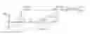
FIG. 1 is a system structure drawing for double-fed wind turbine-infinite system under the PSCAD/EMTDC of the present invention;

FIGS. 2a and 2b are the tendency charts for eigenvalues of the system mode while T_issc is changing of the present invention;

FIGS. 3a and 3b are the tendency charts for eigenvalues of the system mode while K_pssc is changing of the present invention;

FIGS. 4a and 4b are the tendency chart for eigenvalues of the system mode while L is changing of the present invention; and

FIG. 5 is a flow chart of the method to improve disturbance stability after double-fed unit gets access to a system according to the present invention.

SPECIFIC EMBODIMENTS OF THE PRESENT INVENTION

With reference to the drawings and embodiments, the present invention is illustrated in details below. It should be noted that the following illustrations are only examples, but not to limit the range and applications of the present invention.

The present invention adopts the model that is commonly used in researching characteristics of grid-connected operation of double-fed unit in PSCAD/EMTDC: DFIG_—2010_—11 (WIND FARM Vector Controlled Doubly-Fed Induction Generator) as a template to make the following improvements on this model:

1) adjusting reference frequency of the system from 60 Hz to 50 Hz;
2) removing “crowbar” circuit to make it suitable for small disturbance stability analysis after double-fed unit connects to the grid.

This model is double-fed wind turbine-infinite system. Correctness and practicability of the present invention will be verified with this model below. The system structure of this model shall refer to FIG. 1.

In Step 1, system matrix A′ is formed in the following process:

First, building a state equation and an output equation of the double-fed unit. The system state equation is expressed as:

ω . m ′ = 1 T j  ( C p  A blade  ρ   v 3 2  S B  ω m ′ - γ   u s  L m  i qr α   L s  S B - D   ω m ′ )    ω . ref ′ = - 1 T v  ω . ref ′ + 1 λ eq   T v  v   i . qr = ( T i   2 - DK p   2 T j )  ω m + K p   2  kv 3 T j  ω m - ( T i   2 - K p   2 T v )  ω ref - K p   2  γ   u s0  L m α   T j  S B  L s  i qr - K p   2 λ eq  T v  v   i . dr = α  T il  L s α   L s + K pl   γ   u s  L m  [ Q ref - γ   u s  L s  ( i dr  L m α - u s ω s ) ]   x . 1 = 1 T x  ( u dc - x 1 )   i . 1  dref = ( K pcvc T x - T icvc )  x 1 - K pcvc T x  u dc + T icvc  u dcref   u . 1  dref = K pssc  ( K pcvc T x - T icvc )  x 1 + T issc  i 1  dref - K pssc L  u 1  dref + ( K pssc  R L - T issc )  i 1  d - K pssc  K pcvc T x  u dc + K pssc  T icvc  u dcref   i . 1  d = 1 L  u 1  dref - R L  i 1  d    u . 1  qref = ( K pssc  R L - T issc )  i 1  q - K pssc L  u 1  qref + T issc  i 1  qref   i . 1  q = 1 L  u 1  qref - R L  i 1  q   u . dc = γ   u s  [ i 1   d - ( 1 - ω m )  K m α   L s  i qr ] Cu dc ( 13 )

In Equation (13), T_j is an inertia time constant of the generator; ω_s and ω′_m refer to synchronous speed and mechanical speed of the generator; C_p is a rotor power coefficient; A_blade is a blade area; ρ is the air density; v is wind speed; S_B is benchmark capacity of the system; γ is coordinate transformation coefficient; α is stator-rotor turns ratio; u_s is phase voltage amplitude of generator stator; L_s and L_m refer to generator stator self-inductance, stator-rotor mutual inductance and generator rotator self-inductance; D is generator damping coefficient; ω′_ref is reference wind speed used to realize MPT; λ_eq is equivalent tip speed ratio; T_v and T_x refer to time constants during inertia loop; i_dr and i_qr refer to the current of rotator at axis “d” and axis “q”; i_1d and i_1q refer to the current of grid-side converter at axis “d” and axis “q”; R and L refer to converter resistance and reactance; K_p1, T_i1, K_p2, T_i2, K_pcvc, T_icvc, K_pssc and T_issc are PI controller parameters; u_dcref, u_dc and x₁ refer to reference value, actual value and measured value of DC voltage; u_1dref and u_1qref refer to inner ring PI output of grid-side controller; i_1dref and i_1qref refer to outer ring PI output of grid-side controller; C is a DC capacitor.

The output equation is expressed as:

P g = 1.5  u s  ( L m  i qr α   L s - i 1  d )   Q g = - 1.5  u s  ( au s - ω s  L m  i dr αω s  L s - i 1  q ) ( 14 )

The power flow equation of the system is expressed as:

P_g=U²G_line−UE(G_line cos θ+B_line sin θ)

Q_g=U²B_line−UE(G_line sin θ−B_line cos θ)  (15)

In Equation (15), U and θ refer to an effective value and a phase angle of a high-side voltage of a transformer; E is an effective value of a line voltage of an infinite electric power bus; G_line and B_line refer to overall equivalent conductance and susceptance of the transformer and line.

Referring to the method in (2)-(3), linearizing and organizing Equations (13)-(15) at steady-state operation point, it can be concluded as:

A′=A+B(F−D)⁻¹(C−E)  (16)

wherein, state variable Δx, input variable Δu and output variable Δy can be expressed as:

Δx=[Δω*_mΔω*_refΔi_drΔi_qrΔx₁Δi_1drefΔu_1drefΔi_1dΔu_1drefΔi_1qΔu_dc]^T

Δu=[Δu_sΔθ]^T

Δy=[ΔP_gΔQ_g]^T

The matrix that corresponds to Equation (16) is shown as:

A = [ Δ  ω . m * a 0101 0 0 a 0104 0 0 0 0 0 0 0 Δ  ω . ref * 0 a 0202 0 0 0 0 0 0 0 0 0 Δ  i . dr 0 0 a 0303 0 0 0 0 0 0 0 0 Δ  i . qr a 0401 a 0402 0 a 0404 0 0 0 0 0 0 0 Δ  x . 1 0 0 0 0 a 0505 0 0 0 0 0 a 0511 Δ  i . 1  dref 0 0 0 0 a 0605 0 0 0 0 0 a 0611 Δ  u . 1  dref 0 0 0 0 a 0705 a 0706 a 0707 a 0708 0 0 a 0711 Δ  i . 1  d 0 0 0 0 0 0 a 0807 a 0808 0 0 0 Δ  u . 1  dref 0 0 0 0 0 0 0 0 a 0909 a 0910 0 Δ  i . 1  q 0 0 0 0 0 0 0 0 a 1009 a 1010 0 Δ  u . dc a 1101 0 0 a 1104 0 0 0 a 1108 0 0 a 1111 ]    Δω m * Δω ref *  Δ  i dr  Δ  i qr Δ  x 1  Δ  i 1  dref Δ  u 1  dref Δ  i 1  d Δ  u 1  dref Δ  i 1  q Δ  u dc

The subscript “₀” represents steady-state value of relevant variable and superscript “*” represents per unit value. The corresponding matrix elements are shown as:

a 0101 = - 1 T j  ( kv 3 ω m   0 2 + D ) , a 0104 = - γ   u s   0  L m α   T j  S B  L s , a 0202 = - 1 T v , a 0303 = - γ   T i   1  u s   0  L m α   L s + K p   1  γ   u s   0  L m , a 0401 = T i   2 - K p   2  D T j - K p   2  kv 3 T j  ω m   0 2 , a 0402 = K p   2 T v - T i   2 , a 0404 = - K p   2  γ   u s   0  L m α   T j  S B  L s  a 0505 = - 1 T x , a 0511 = 1 T x , a 0605 = K pcvc T x - T icvc , a 0611 = - K pcvc T x , a 0705 = K pssc  ( K pcvc T x - T icvc ) , a 0706 = T issc , a 0707 = - K pssc L , a 0708 = K pssc  R L - T issc , a 0711 = - K pssc  K pcvc T x , a 0807 = 1 L , a 0808 = - R L , a 0909 = - K pssc L , a 0910 = K pssc  R L - T issc , a 1009 = 1 L , a 1010 = - R L , a 1101 = γ   u s   0  L m  i qr   0 α   Cu dc   0  L s , a 1104 = γ   u s   0  L m  ( 1 - ω m   0 ) α   Cu dc   0  L s , a 1108 = γ   u s   0  Cu dc   0 , a 1111 = - γ   u s   0  [ i 1  d   0 - ( 1 - ω m   0 )  L m  i qr   0 α   L s ] Cu dc   0 2 

wherein, m is the ratio between effective value of high-side voltage of transformer and phase voltage amplitude of a generator stator. k_T is the k_T boosting transformer ratio.

A part of system parameters of this simulation model are shown in the following table.

TABLE 1
System Parameter Table

					Value/
Parameter	Value/unit	Parameter	Value/unit	Parameter	unit
Rs	0.0054 p.u.	Rr	0.00607 p.u.	Lsσ	0.1 p.u.
Lrσ	0.11 p.u.	Lm	4.5 p.u.	ωs	314.15
					rad/s
D	0.0001 p.u.	Ablade	5026.55 m2	P	1.225
					kg/m3
Cp	0.28	C	0.0078 F	L	1 mH
Kpssc	1 p.u.	Tissc	0.1 p.u.	Tx	0.04 μs

Analysis results of eigenvalues of system matrix A′ should refer to Table 2.

TABLE 2
Analysis Results of Eigenvalues of A′

			Oscillation	Most	Second
		Damping	frequency/	relevant	relevant
No.	Eigenvalue	ratio	Hz	variable	variable

λ1	−1214.3316	1	0	u1dref	i1d
λ2,3	−4.8122 ± 130.8084i	0.0368	20.8188	udc	i1d
λ4	−1199.9167	1	0	u1qref	i1q
λ5,6	−0.7275 ± 1.0064i	0.5858	0.1602	ω*m	iqr
λ7	−0.0010	1	0	x1
λ8	−0.1000	1	0	i1dref
λ9	−0.0833	1	0	i1q	u1qref
λ10	−20	1	0	ω*ref
λ11	−0.8193	1	0	idr

From the analysis results of Table 2, all the eigenvalues of the system matrix A′ have negative real part, which represents the system is of small disturbance stability at this steady-state operation point. However, upon careful observation, it can figure out that the eigenvalues that correspond to evanescent modes λ₇, λ₈ and λ₉ are close to origin, so that unstability is easy to happen. Besides, damping of oscillation mode λ_2,3 is small, which is only 0.0368, so that it is weak damping mode. For the above modes, it can figure out that small disturbance stability margin of this system is relatively low and when steady-state operating point shifts, unstability might happen.

After finding out the mode needs to be focused, taking Step 2 to solve sensitivities of the modes λ_2,3, and λ₇, λ₈ and λ₉ to the nonzero elements in A′. For the expression of elements, the state matrix A can be used instead. Detailed results should refer to Table 3.

TABLE 3
Sensitivity of Weak Damping Mode to the Elements in A′

		Corresponding
Mode	Element	expression in A	Sensitivity	Abandon or not
λ2,3	a0706′	Tissc	0.4950 − 0.0716i	No
	a0708′	K pssc  R L - T issc	0.4028 − 0.1041i	No
	a1106′	0	−0.0013 + 0.9443i	Yes
λ7	a0505′	- 1 T x	1.0011	No
	a0511′	1 T x	1.0011	No
λ8	a0606′	0	1.0013	Yes
	a0706′	Tissc	−1.0015	No
	a0806′	0	−1.0014	Yes
λ9	a0909′	- K pssc L	0.8334	No
	a0910′	K pssc  R L - T issc	−0.8334	No

It can be concluded from Table 3 that T_issc, K_pssc, T_x, L and R are relatively more sensitive to the weak damping mode happened to this system. Conditions about the changes of different system modes are researched below when the above parameters change (the initial parameter values should refer to Table 1):

1) Conditions about the Changes of System Eigenvalues when T_issc Changes

Taking the change interval of T_issc as [0, 10], selecting parameter nodes as T_issc=0.1, 1, 5, 10 and observing simulation steady-state solution. It is concluded from the results that when T_issc changes, simulation steady-state solution is basically unchanged. Take ΔT_issc=1, change track of system eigenvalues should refer to FIGS. 2a and 2b.

It can be concluded from FIGS. 2a and 2b that when T_issc=0, the system will have a zero eigenvalue. With T_issc increases, damping ratio λ_2,3 of oscillation mode will decrease slightly and damping of evanescent modes λ₈ and λ₉ will increase obviously. As when T_issc increases, damping ratio of oscillation mode λ_2,3 decreases little, but damping of evanescent modes λ₈ and λ₉ increases obviously, so that T_issc can be increased properly to improve small disturbance stability of the system, taking {circumflex over (T)}_issc=10.

2) Conditions about the Changes of System Eigenvalues when K_pssc Changes

Replacing original T_issc with {circumflex over (T)}_issc=10 obtained from 1), setting the change interval of K_pssc as [0, 10], selecting parameter nodes as K_pssc=0.1, 1, 5, 10 and observing simulation steady-state solution. It is concluded from the results that when K_pssc changes, simulation steady-state solution is basically unchanged. Setting ΔK_pssc−1, the changing track of the system eigenvalues should refer to FIGS. 3a and 3b.

It can be concluded from FIGS. 3a and 3b that when K_pssc=0, positive real part happens to oscillation mode λ_2,3 (λ_2,3=35.0110±16.4581i), the steady-state of the system becomes unstable and evanescent modes λ₁ and λ₄ become a group of oscillation modes. With K_pssc increases, damping of oscillation mode λ_2,3 will increase, but the eigenvalues that correspond to weak evanescent modes λ₈ and λ₉ move from negative real axis to origin point and its degree of stability decreases. Thus, if K_pssc is too big or too small, the degree of stability of the system will be decreased. It can be figured out from FIGS. 3a and 3b that when K_pssc>3, damping of mode λ_2,3 will increase slowly, but λ₈ and λ₉ still move to the origin point, so that take {circumflex over (K)}_pssc=2.

3) Conditions about the Changes of System Eigenvalues when T Changes

It can be concluded from Table 3 that T_x is only highly sensitive to λ₇. T_x is an inertia time constant while measuring DC voltage, the value of which is small. Setting the change interval as [0.01,0.1], it can be concluded from the results that when T_x changes, the simulation stability solution is basically unchanged. When ΔT_x=0.01, from simulation results, it figures out that the system eigenvalue that changes T_x is also basically unchanged, which indicates that weak damping of mode λ₇ is unrelated to system parameters and it is caused by system structure. Thus, if value of T_x does not change, keeping T_x=0.04.

4) Conditions about the Changes of System Eigenvalues when L Changes

L is the equivalent conversion inductance of a grid-side converter, setting change interval of L as [0.5,2] mH, selecting parameter nodes as L=0.5, 1, 1.5, 2 and observing simulation steady-state solution. It is concluded from the results that when K_pssc changes, simulation steady-state solution is basically unchanged. Setting ΔL=0.1 mH, the change track of system eigenvalues should refer to FIGS. 4a and 4b.

It can be concluded from FIGS. 4a and 4b that with L increases, damping of oscillation mode λ_2,3 will decrease obviously and damping ratio also reduces; eigenvalue that corresponds to evanescent mode λ₉ tends to move away from an imaginary axis, but it is not obvious and can be ignored; strong evanescent modes λ₁ and λ₄ move towards the origin rapidly and damping decreases, but it still does not belong to strong damping and influence little on system stability. Therefore, if it is allowed, L is smaller, the stability margin of the system is higher. Take {circumflex over (L)}=0.5 mH here.

5) Conditions about the Changes of System Eigenvalues when R Changes

R is the AC side equivalent resistance of a grid-side converter. Upon analysis, it indicates that when R>0.5Ω, oscillation will happen to the system; when R<0.5Ω, value of R has very little influence on system eigenvalues. On the basis of the above conclusions, take {circumflex over (R)}=0.2Ω.

Until now, optimization for the parameters that correspond to the four concerned modes is completed. Table 4 is about the comparison between key mode eigenvalues of initial parameters and optimal parameters of the system. It can be concluded through analyzing the above contents, T_x and R influence little on eigenvalues. Thus, in Table 4, initial parameters and optimal parameters are set as T_x=0.04 and R=0.2Ω.

TABLE 4
Comparison between Key Mode Eigenvalues of Initial Parameters
and Optimal Parameters

Parameter

	Initial parameter	Optimal parameter
Mode	Tissc = 0.1 {circumflex over (K)}pssc = 1 {circumflex over (L)} = 1 mH	{circumflex over (T)}issc = 10 {circumflex over (K)}pssc = 2 {circumflex over (L)} = 0.5 mH
λ2,3	−4.8122 ± 130.8084i	−9.6379 ± 137.1746i
λ7	−0.0010	−0.0010
λ8	−0.1000	−5.0028
λ9	−0.0833	−4.5502

It can be concluded from Table 4 that except mode λ₇, damping of other dominant modes has been raised for a certain extent. For λ₇, its weak damping is not caused for selecting improper parameters, so that it needs to be improved through changing system control structure or adding other control devices; for oscillation λ_2,3, its damping has been raised from 0.0368 to 0.0701; λ₈ and λ₉ have changed from weak damping mode to strong damping mode and small disturbance stability margin of the system has been improved obviously.

What is said above has totally verified that while researching the weak damping mode generated after double-fed unit gets access to power grid, system damping can be effectively improved without adding other control means through optimizing system parameters with sensitivity analysis. Compared with traditional optimization methods. The present invention will greatly decrease unnecessary calculated amount and improve efficiency.

This test system is only a preferred embodiment of the present invention, but protection scope of the present invention is not confined to the embodiment. Any changes or replacements that the person of ordinary skill in the art can figure out easily within the technical range disclosed by the present invention should be included in the protection scope of the present invention.