Imaging Device and Method for Sensing Media Type
US20160044195A1
2016-02-11
14/295,838
2014-06-04
Abstract:
An operational imaging device and method for sensing a media type in a predetermined media set using a predetermined set of media type determining equations solved using measured values for a set of N variables measured by an operational sensor set in the operational imaging device. The solution of the equation set determines a media type. After a media type is determined, one or more operational parameters of the imaging device is selected for processing of a sheet of the determined media type. The equation set is generated by a training system using a classifier training engine. A plurality of training data sets containing measured variable values for each media type is collected under various conditions by a training sensor set that measures the set of N variables. After generation, the media type determining equation set is stored in memory of the operational imaging device.
Inventors:
- Niko Jay Murrell 23 🇺🇸 Lexington, KY, United States
- Julie Ann Gordon Whitney 2 🇺🇸 Gerogetown, KY, United States
- Ryan Thomas Bradley 2 🇺🇸 Lexington, KY, United States
- Nikhil Bajaj 15 🇺🇸 West Lafayette, IN, United States
Interested in similar patents?
Get notified when new applications in this technology area are published.
Classification:
H04N1/00724 » CPC main
Scanning, transmission or reproduction of documents or the like, e.g. facsimile transmission; Details thereof; Detecting the presence, position or size of a sheet or correcting its position before scanning; Object of the detection Type of sheet, e.g. colour of paper or transparency
G06K15/021 » CPC further
Arrangements for producing a permanent visual presentation of the output data, e.g. computer output printers using printers Adaptations for printing on specific media
G06K15/102 » CPC further
Arrangements for producing a permanent visual presentation of the output data, e.g. computer output printers using printers by matrix printers using ink jet print heads
G06K15/4065 » CPC further
Arrangements for producing a permanent visual presentation of the output data, e.g. computer output printers; Details not directly involved in printing, e.g. machine management, management of the arrangement as a whole or of its constitutive parts Managing print media, e.g. determining available sheet sizes
H04N1/00708 » CPC further
Scanning, transmission or reproduction of documents or the like, e.g. facsimile transmission; Details thereof; Detecting the presence, position or size of a sheet or correcting its position before scanning; Object of the detection Size or dimensions
H04N1/00729 » CPC further
Scanning, transmission or reproduction of documents or the like, e.g. facsimile transmission; Details thereof; Detecting the presence, position or size of a sheet or correcting its position before scanning Detection means
H04N2201/0094 » CPC further
Indexing scheme relating to scanning, transmission or reproduction of documents or the like, and to details thereof; Types of the still picture apparatus Multifunctional device, i.e. a device capable of all of reading, reproducing, copying, facsimile transception, file transception
H04N2201/0082 » CPC further
Indexing scheme relating to scanning, transmission or reproduction of documents or the like, and to details thereof; Types of the still picture apparatus Image hardcopy reproducer
H04N2201/0081 » CPC further
Indexing scheme relating to scanning, transmission or reproduction of documents or the like, and to details thereof; Types of the still picture apparatus Image reader
H04N1/00 IPC
Scanning, transmission or reproduction of documents or the like, e.g. facsimile transmission; Details thereof
G06K15/00 IPC
Arrangements for producing a permanent visual presentation of the output data, e.g. computer output printers
G06K15/10 IPC
Arrangements for producing a permanent visual presentation of the output data, e.g. computer output printers using printers by matrix printers
G06K15/02 IPC
Arrangements for producing a permanent visual presentation of the output data, e.g. computer output printers using printers
G06K15/14 » CPC further
Arrangements for producing a permanent visual presentation of the output data, e.g. computer output printers using printers by electrographic printing, e.g. xerography; by magnetographic printing
Description
CROSS REFERENCES TO RELATED APPLICATIONS
This patent application is related to the U.S. patent application Ser. No. ______, filed June DAY, 2014, entitled “Imaging Device And Method For Determining Operating Parameters” (docket no. P611-US2) and assigned to the assignee of the present application.
STATEMENT REGARDING FEDERALLY SPONSORED RESEARCH OR DEVELOPMENT
None.
REFERENCE TO SEQUENTIAL LISTING, ETC.
None.
BACKGROUND
1. Field of the Disclosure
The present disclosure relates generally to imaging devices, and, more particularly, to those systems and methods for sensing types or classes of media.
2. Description of the Related Art
Incorrectly setting media type is a well-documented problem for users of imaging devices, such as electrophotographic printers. Setting media properties correctly is difficult for three primary reasons. First, properly identifying media is a subjective decision. Second, paper setting menus are sometimes difficult to locate and navigate. Third, classification of equivalent media is inconsistent. Additionally, media moisture content and environmental factors may invalidate correctly chosen settings. As a consequence of this, it is common for imaging devices to operate suboptimally.
There are consequences to improperly selected media type settings. The imaging device relies upon media type settings to control media handling, transfer, fusing, and finishing operations. Common failures related to improper media type settings include poor print quality, poor fusing, hot or cold offset, paper jams, media damage, component wear, and wrapping of the fuser by the media. This leads to user dissatisfaction.
To address this problem, several solutions that incorporate some form of printer control based upon sensed media properties have been developed. Prior art sensor implementations describe devices that measure a single media property, or at most, a few specific properties, such as optical transmission and impedance, to provide limited media identification. Prior art control schemes are limited in scope and are based upon an incomplete characterization of the media. Such prior art systems still rely upon user input and lack a holistic approach. An idealized, fully-featured sensing scheme would take a single, direct measurement of all relevant intrinsic media properties and use this information to model and control the imaging device. However, the number of intrinsic property measurements required to adequately control an imaging device, such as an electrophotographic printer, without user input is prohibitive as this approach is neither cost nor space efficient and requires a large number of sensors. Prior art sensing schemes have been incomplete because they have failed to measure some number intrinsic properties of the media needed to more accurately determine the media type.
It would be advantageous to be able to select a minimum set of sensors for an imaging device based on its intended application, such as retail use, office use, or a general purpose device suitable for a wide range of tasks; measure an extrinsic media property in lieu of several independent intrinsic media properties, and, then determine media type without the need for user intervention.
SUMMARY
Disclosed is a method of media type sensing for use in an operational imaging device such as an electrophotographic printer. The method comprises in one aspect: establishing a media set comprising a plurality of media types M to be used in the operational imaging device; determining a number of variables N needed to determine each media type in the media set; providing a training sensor set for measuring each of the N variables and providing corresponding output signal therefor; using the training sensor set to measure the N variables with a known sample of each media type in the media set and a training imaging device to create a corresponding training data set for each media type in the media set, wherein the measuring includes taking multiple measurements of each of the N variables; inputting each training data set for each media type into a classifier training engine; and generating, using the classifier training engine, a media type determining equation for each media type incorporating corresponding N variable terms to create a set of M media type determining equations for use with an operational set of sensors corresponding to the training set sensors.
The method in another aspect, in an operational imaging device, comprises: storing in a memory the set of M media type determining equations; providing an operational sensor set for operable communication with the operational imaging device, the operational sensor set measuring a value of each variable in the set of N variables and providing corresponding output signals for the measured N variables for a sheet of media to be processed; converting the received output signals into the N measured normalized variable values; solving the set of M media type determining equations using the N measured normalized variable values to determine a media type from the media set for the media sheet to be processed; and, selecting, based upon the determined media type, from a look up table at least one operational parameter for the operational imaging device.
The method in another aspect includes the measuring of multiple measurements of each of the N variables by the training sensor set occurs at a plurality of predetermined temperature and relative humidity combinations. The set of N variables comprises at least two variables selected from the group comprising: electrical impedance magnitude, electrical impedance phase, contact resistance, capacitance, optical transmission mean, optical transmission deviation, optical spectral reflectance, optical diffuse reflectance, bending stiffness, acoustic transmission, temperature, media size, relative humidity, media feed motor current, fuser temperature, transfer current, transfer voltage, media holes, preprinted areas, media color, multilayer media, RFID signal, magnetic field, MICR, and further wherein the operational sensor set includes sensors for measuring the at least two selected variables.
BRIEF DESCRIPTION OF THE DRAWINGS
The above-mentioned and other features and advantages of the disclosed embodiments, and the manner of attaining them, will become more apparent and will be better understood by reference to the following description of the disclosed embodiments in conjunction with the accompanying drawings.
FIG. 1 is a schematic representation of a training system used with the presently disclosed system and methods.
FIG. 2 is an illustration of training data sets.
FIG. 3 is a schematic representation of an operational device employing the presently disclosed system and methods.
FIGS. 4-5 illustrate two types of operational parameter ranges schemes.
FIG. 6 illustrates the use of a matrix of media type determining equation sets to handle faulty sensors.
FIG. 7 is a simplified block diagram of the present method of using media type determining equation sets in an operational imaging device to determine a media type.
FIGS. 8A-8B are simplified block diagrams of the present method providing for operation in the event of a faulty sensor in an operational imaging device.
DETAILED DESCRIPTION
It is to be understood that the present disclosure is not limited in its application to the details of construction and the arrangement of components set forth in the following description or illustrated in the drawings. The present disclosure is capable of other embodiments and of being practiced or of being carried out in various ways. Also, it is to be understood that the phraseology and terminology used herein is for the purpose of description and should not be regarded as limiting. The use of “including,” “comprising,” or “having” and variations thereof herein is meant to encompass the items listed thereafter and equivalents thereof as well as additional items. Unless limited otherwise, the terms “connected,” “coupled,” and “mounted,” and variations thereof herein are used broadly and encompass direct and indirect connections, couplings, and mountings. In addition, the terms “connected” and “coupled” and variations thereof are not restricted to physical or mechanical connections or couplings.
Spatially relative terms such as “top”, “bottom”, “front”, “back”, “rear”, “side” “under”, “below”, “lower”, “over”, “upper”, and the like, are used for ease of description to explain the positioning of one element relative to a second element. These terms are intended to encompass different orientations of the device in addition to different orientations than those depicted in the figures. Further, terms such as “first”, “second”, and the like, are also used to describe various elements, regions, sections, etc. and are also not intended to be limiting. Like terms refer to like elements throughout the description.
As used herein, the terms “having”, “containing”, “including”, “comprising”, and the like are open ended terms that indicate the presence of stated elements or features, but do not preclude additional elements or features. The articles “a”, “an” and “the” are intended to include the plural as well as the singular, unless the context clearly indicates otherwise.
In addition, it should be understood that embodiments of the present disclosure include both hardware and electronic components or modules that, for purposes of discussion, may be illustrated and described as if the majority of the components were implemented solely in hardware. However, one of ordinary skill in the art, and based on a reading of this detailed description, would recognize that, in at least one embodiment, the electronic based aspects of the invention may be implemented in software. As such, it should be noted that a plurality of hardware and software-based devices, as well as a plurality of different structural components may be utilized to implement the invention. Furthermore, and as described in subsequent paragraphs, the specific mechanical configurations illustrated in the drawings are intended to exemplify embodiments of the present disclosure and that other alternative mechanical configurations are possible.
It will be further understood that each block of the diagrams, and combinations of blocks in the diagrams, respectively, may be implemented by computer program instructions. These computer program instructions may be loaded onto a general purpose computer, special purpose computer, or other programmable data processing apparatus to produce a machine, such that the instructions which execute on the computer or other programmable data processing apparatus may create means for implementing the functionality of each block or combinations of blocks in the diagrams discussed in detail in the descriptions below.
These computer program instructions may also be stored in a non-transitory, tangible, computer readable storage medium that may direct a computer or other programmable data processing apparatus to function in a particular manner, such that the instructions stored in the computer readable storage medium may produce an article of manufacture including an instruction means that implements the function specified in the block or blocks. Computer readable storage medium includes, for example, disks, CD-ROMS, Flash ROMS, nonvolatile ROM and RAM. The computer program instructions may also be loaded onto a computer or other programmable data processing apparatus to cause a series of operational steps to be performed on the computer or other programmable apparatus to produce a computer implemented process such that the instructions that execute on the computer or other programmable apparatus implement the functions specified in the block or blocks. Output of the computer program instructions, such as the process models and the combined process models, as will be described in greater detail below, may be displayed in a user interface or computer display of the computer or other programmable apparatus that implements the functions or the computer program instructions.
The term “image” as used herein encompasses any printed or digital form of text, graphic, or combination thereof. The term “output” as used herein encompasses output from any printing device such as color and black-and-white copiers, color and black-and-white printers, and multifunction devices that incorporate multiple functions such as scanning, copying, and printing capabilities in one device. Such printing devices may utilize ink jet, dot matrix, dye sublimation, laser, and any other suitable print formats. The term button as used herein means any component, whether a physical component or graphic user interface icon, that is engaged to initiate an action or event.
Referring now to FIG. 1, a schematic representation of a training system 10 used with present media type sensing system is illustrated. Included in training system 10 is a trainer 12 that provides firmware that will be incorporated into one or more operational imaging devices, generally indicated 50, operational imaging devices 50-1 through 50-K as shown. Also included in training system 10 is a training sensor set 14, a training media set 16 comprised of M different media types, 16-1-16-M, a robot 18, a training imaging device 22, and imaging device subsystems 24. A robot 18 or robotic job processor 18 is simply a machine designed to perform a function of an operational imaging device 50. For example, where the operational imaging device 50 is an electrophotographic printer, training system 10 may use a fuser robot that performs fusing, a transfer station robot that performs toned image transfer to a media sheet, or a media feed robot that emulates feeding media sheets. Training sensor set 14 is used to measure N different variables related to each media type in the training media set 16 or related to the traning imaging device 22 or its subsystems 24 to form training data sets for each media type. The training imaging device 24 would be an imaging device that is substantially the same as an operational imaging device 50 that would be used by a customer. However, the training imaging device 22 would be used in a laboratory or test enclosure so that environmental conditions could be controlled when making measurements as described herein.
A training sensor set 14, consisting of a predetermined collection of sensors, provides data measurement points to trainer 12. The types and number of sensors used will be described below and will vary dependent upon the media types included in training media set 16, the ambient conditions 20 to be measured, the type of robots 18 and training imaging device 22 used, and functional requirements and customer requirements for the operational imaging devices 50. The training sensor set 14 is used in conjunction with the training media set 16, comprised of samples of M different media types and provides multiple data points for each variable in a predetermined set of N variables. Possibly included in the set of N variables that training sensor set 14 measures, as illustrated by the reflecting arrows, are those relevant to each media type M in the media set 16; ambient conditions, indicated by cloud 20, such as temperature and relative humidity where the training media set 16 is located, and variables relevant to the operational imaging device 50 such as electrical, thermal and mechanical properties measured using the robots 18 or training imaging device 22. An operational imaging device designer chooses variables that will provide a resolution sufficient to determine each media type M within the training media set 16. The chosen variables N relevant to the distinguishing the media types in the training media set 16 are empirically determined and verified. For a given family of operational imaging devices 50, the chosen N variables to be measured using subsystems equivalent to subsystems common to each member of a given family of operational imaging devices 50. These subsystems may be provided in a training imaging device 22 or may be individually provided subsystems, generally indicated 24, such a transfer station 24-1, fuser 24-2 or media feed system 24-3, etc. It will be noted that each media type M is tested with each robot 18, the training imaging device 22, if present, or subsystems 24 at several different ambient conditions and measurements are also taken at a plurality of locations within the borders of the media sheet. The use of robots 18 and/or subsystems 24 may obviate the need to use a training imaging device 22.
Training sensor set 14 comprises direct sensors 14-1, indirect sensors 14-2 and subsystem response sensors 14-3 for one or more subsystems that will be present within the operational imaging device 50. Such subsystems include a fuser, a toner transfer station, a media feed system, and a finisher, which may also be termed a processing device.
Direct sensor measurements are of a characteristic of the media. These direct measurements include, but are not limited to, optical, electrical impedance, reflectance, thermal capacitance, etc. A more extensive list of direct sensor measurements that may be used with the present system 10 and operational imaging devices 50-1-50-K is provided in Table 3 below.
Indirect measurements include, but are not limited to, temperature, relative humidity, and/or the desired machine state, e.g., process speed. When such indirect measurements are made, each media type in the media set and each imaging device subsystem are measured at the desired indirect measurement points. For example, when temperature and relative humidity are being measured, each media type in the training media set 16 and each imaging device subsystem 24 are measured at several different temperature and humidity points, such as, for example, 22° C. at 50% relative humidity, 25.6° C. at 80% relative humidity, and 15° C. at 8% relative humidity. These temperature and humidity points are environments in which operational imaging devices 50 may be placed. Multiple samples of each media type are measured in these different environments to generate the training data set 26. Other temperature and humidity conditions may also be measured.
Subsystem response measurements include change of fuser temperature occurring for each media type in the training media set 16 as they are fed through the fuser, change in transfer nip voltage or current occurring for each media type as they are fed through the transfer nip of the transfer station, media feed motor current for each media type as they are fed through the media path, and/or media location within the media path. Again these measurements may be taken at several different temperatures and relative humidity values and are included in the training data set 26.
A single sensor in the training sensor set 14 may provide data for two or more variables in the set of N variables. For example, an impedance sensor may provide both magnitude and phase data points. The output of each sensor in the training sensor set 14 may be conditioned and normalized by trainer 12 so that M data training sets 26 contain normalized data points. This helps to improve performance of training system 10.
The data for the N variables for each media type M in the training media set 16 is collected in a data set, generally designated 26, for each media type M, training data sets 26-1 through 26-M as shown. For data in the training data sets 26 the media type or class to which that data belongs is known. For example, should training media set 16 have three media types 16-1-16-3, three data sets 26-1-26-3 would be collected. It will be appreciated that the number of data points within each data set 26 will number in the thousands. In general, as the media types M to be sensed in operational imaging devices 50 increases in number, the number of variables N measured increases so that each media type M may be determined. The measurements taken for the training data sets 26 may also account for sensor aging, sensor variability, media variability, imaging device subsystem variability to achieve a robust set of media type determining equations flexible enough to handle variability in the operational sensor set 52, in the media types and the operational imaging devices 50. Further, multiple instances of the same sensor and multiple instances of the same type of media sheet may be used when populating the training data sets 26.
As used herein, the N variables in each data set 26 for each media type M includes the variables types previously described such as temperature, relative humidity and corresponding imaging device variables, all as selected for inclusion in the predetermined set of N variables. FIG. 2 illustrates a 4×4 matrix of three data sets 26-1-26-3 for three media types—polyvinyl M1, cardstock M2 and plain paper M3. Note that the data in FIG. 2 has not been normalized. The data points for polyvinyl M1 are indicated by a star, those for cardstock M2 by a triangle, and those for plain media M3 by a cross. For the data sets 26-1-26-3, the four variables chosen by the imaging device designer to be measured are bending N1 in Watts, impedance magnitude N2 in ohms, impedance phase N3 in degrees and reflectance or gloss N4 in Volts. Clustering of the data points for each of the media types M1-M3 can readily be seen. These three data sets 26-1-26-3 would be processed by trainer 12 to produce a media type determining equation set 40 having three media type determining equations.
For the purposes of developing a media type determining equation that can successfully classify media type given the different variable input magnitudes, the measured sensor values are normalized prior to training. This is because units of Ohms have no physical comparison to units of optical transmission, degrees of temperature, or percent relative humidity, etc. The goal is to compare how the media is changing with respect to its physical properties and by normalizing the inputs to the same order of magnitude this can be more easily achieved. Before training, these input values are normalized such that the magnitudes of each of the inputs are roughly equivalent over the range expected by the operational imaging devices 50, the media types expected to be used, expected environments of use, and one or more desired machine states, for example, 40 page per minute (ppm) process speed or 70 ppm process speed. The measured values provided by the operational sensor sets 52 would also be normalized prior to controllers 51 solving the media type determining equations sets 40.
The M data sets 26 of N variables each are fed into a classifier training engine 30. Using the M data sets 26, classifier training engine 30 produces as an output a media type determining equation set 40 containing M media type determining equations, where M is the number of media types and N is the number of variables. It should be understood that the number of variables N does not have to equal the number of media types M. The media type determining equation set 40 will be replicated, 40-1 through 40-K as shown, and installed into each corresponding operational imaging device 50-1-50-K.
Classifier training engine 30 uses a supervised machine learning algorithm used to map inputs (sensed media variables or properties like bending stiffness, electrical impedance, acoustic transmittance, optical reflectance, etc.) to a media type or class. In supervised learning, for a given input data set, the correct output is known. For data in the training data sets 26 the media type or class to which that data belongs is known. With a classifier training engine 30, results are predicted in a discrete output and input variables are mapped to discrete classes or type—here discrete media types. Once the media type determining equations are formed, these equations, when placed in the operational imaging devices 50, take measured variable values from the operational sensor set 52 as inputs and use them to determine the best class (i.e. media type). The measured variable values are also termed instances. Classification into one of the several media types may be done by multiclass classification or by combining multiple binary classifiers that deal with only two classes at a time. A classification scheme is advantageous since programs in many existing imaging device controllers are based upon a discrete categorization of media into type, weight, and roughness.
Classifier training engine 30 may be one of well known classification engines as known in the art that analyze data and recognize patterns for classification. These include a support vector engine 30-1, a neural network 30-2, a quadratic classifier 30-3, a Bayesian network 30-4, or a learning vector quantizer 30-5. Classifier training engine 30 operates on the data sets 26-1-26-M to produce the multi-variable media type determining equation set 40. The media type determining equation set 40 may be constructed many different ways. In one embodiment (created using regression techniques), it resembles a higher order multivariable polynomial. In another embodiment (created using neural networks), it resembles two theta matrices. The form of the media type determining equation will be determined by the type of classifier training engine used in trainer 12. Note that, once determined, the media type determining equation may be manipulated to take any convenient mathematical form.
Two optional elements are shown in FIG. 1. These are a polynomial consolidator 32 and expert knowledge cost/value weighter 34. Where the equation set 40 comprises polynomial equations, an optional polynomial consolidator 32 may also be provided to operate on each of the M equations in the set of media determining equations 40 to reduce the number of terms in each equation M. Using a polynomial consolidator 32 reduces the number of terms in each polynomial equation in the media type determining media set 40, and, in turn, the memory and processing power needed by controllers 53 in operational imagining devices 50.
An example implementation of polynomial consolidator 32 will now be described. The following nomenclature is a representative notation for when classifier training engine 30 is a support vector machine, which include examples such as Least-Squares Support Vector Machines (LS-SVM) and Fast Support Vector Machines (FSVM) and many others. For the purposes of this illustration of the polynomial consolidator 32 for use in embedded classification systems to be employed in operational imaging devices 50, a LS-SVM is shown the illustrated implementation where:
p: number of variables;
x: current set of measurements to be classified, a vector of length p;
mk: measurement vector from the training data set, with length p, associated with the kth training data point;
αk: weight associated with the kth training data point;
yk: true classification (usually coded +1 or −1, but could be another form) associated of the kth training data point;
b: linear bias offset term; and
N: number of training data points.
The method of arriving at these quantities is as follows: generally, the set of N vectors mk, k=1, . . . , N and their corresponding true classifications yk are arrived at through experimentation or other means of creating example data points that characterize the categories, i.e., the media types, that are to be used in the classification. For example, if one were trying to distinguish a class A and a class B, one might measure the characteristics of examples from class A, and also measure the characteristics of examples from class B. For each example, the characteristic features, or measurements, are aggregated in a corresponding vector mk. N would then be the sum of the number of examples from class A and class B. The weights αk are arrived at through a training process, which differs somewhat for different classification algorithms, and, for the purposes of polynomial consolidation, the method by which they are attained is not important.
The resulting classification function, C(x), may also depend to some degree on the particular classification algorithm. The polynomial consolidation methodology applies to any classification function that one might apply in this manner as long as it is continuous on a bounded interval of interest. By the Weierstrass approximation theorem, it is well known that any function that meets this criteria can be arbitrarily closely approximated by a polynomial function. For example, many implementations of neural network classifiers utilize continuous functions such as the sigmoid function or alternatively the hyperbolic tangent as a key component.
In the LS-SVM with a polynomial kernel implementation the classification function is set for in Eq. 1:
C(x)=sign[Σi=1Nαkyk(mkTx+b)d] Eq. 1
In this form, d is an integer that provides the degree of the polynomial, and the other terms are as described previously. This form of classifier can have very high performance depending on the characteristics of the system in which it is operating. However, the level of performance increases as the value of N increases. If the performance desired is obtained only after using N=1000 or more examples, then in order to compute C(x), 1000 sums must be performed. In addition, the values of αk, yk, b and mk must be stored in memory in order to compute the classification function.
For embedded systems the computational complexity and memory requirement is a significant disadvantage and in many implementations could force the addition of significant cost to a product in order to incorporate the computational power and memory needed to accommodate the classification function. Polynomial consolidation addresses this problem of computational complexity and memory footprint. Instead of evaluating potentially thousands of terms, the function can be represented by a polynomial.
Certainly, each of the N terms would contribute a different function. In the case of the polynomial form mentioned above, in a LS-SVM classifier training engine 30, each of the N terms would contribute a term as shown in Eq. 2:
αkyk(mkTx+b)d Eq. 2
Considering the transposed vector multiplied by another vector is an inner product and assuming the components of mk are [ak, bk, ck, . . . ]T the result is the expression shown in Eq. 3:
αkyk(αkx1+bkx2+ckx3+dkx4 . . . +b)d Eq. 3
This can be expanded via the multinomial theorem's formula, shown in Eq. 4:
( s 1 + s 2 + … + s q ) d = ∑ k 1 + k 2 + … + k q = d ( d k 1 , k 2 , … , k q ) ∏ 1 ≤ j ≤ q x j k j where ( d k 1 , k 2 , … , k q ) = n ! k 1 ! k 2 ! … k q ! , Eq . 4
a binomial coefficient
Once terms are expanded out for each data point, the result is a list of multivariate polynomials where the coefficients are related to αk, yk, b, d and mk, and the variables are the features or measurements of the data point to be classified, namely x1, x2, . . . , xp, with the number of multivariate polynomials being the number of data points used in the classification (the support vectors).
As an example, consider a system with a second order polynomial classifier where there is one sensor, whose value to be classified is x, and three data points m1, m2, m3 that were used to train the classifier. Since it has already been trained, we also have the corresponding weights α1, α2, α3, corresponding true values y1, y2, y3, and corresponding offset number T. The classifier would then have the form shown in Eq. 5:
y=sign [α1y1(m1x+τ)2+α2y2(m2x+τ)2+α3y3(m3x+τ)2] Eq. 5
If we consider the portion within the brackets Eq. 6 results:
α1y1(m1x+τ)2+α2y2(m2x+τ)2+α3y3(m3x+τ)2=α1y1(m12x2+2m1τX+τ2)+α2y2(m22x2+2m2τx+τ2)+α3y3(m32x2+2m3τX+τ2) Eq.6
Due to the multinomial theorem as discussed above, we can then collect like terms in x, resulting in an expression of the form c1x2+c2x+c3. In this case, c1=α1y1m12+α2y2m22+α3y3m32, and similarly the terms can be collected to develop expressions for c2 and c3 and any other constants for the expression.
In this example, in the final product implementation only c1, c2, and c3 need to be stored in order to classify the new data point, and the savings in both memory footprint and computational complexity are significant, decreasing the potential cost of implementing the classification system in operational imaging device 50. While this becomes a complicated process for more training data points and more variables, the method illustrated is a framework for solving the problem, which can be automated using computer algebra systems.
The expert knowledge cost/value weighter 34 may be employed to adjust the weighting of the coefficients in the M media type determining equation set 40. In trainer 12, generally a cost/value function that is being optimized—that is, starting with some initial “guess” of the best weightings for the function, a cost function is evaluated and properties that are uncovered during this evaluation are used to refine the “guesses” of the weight values until an optimal classifier training engine for that form is found. Generally, the cost/value function lends itself well to optimization, and properties such as convexity of the cost function are very desirable as it leads to a well-studied set of optimization solution methodologies. In some instances some “allowable” confusion between categories (i.e. media types) may exist, depending on certain conditions. These conditions could be based on areas or ranges of features, or any other sensor or condition for which an expert may have intrinsic knowledge. This may also be referred to as expert knowledge. When an error between two categories is allowable (i.e., a particular type of mistake made may not invalidate the results of the multiclass classification) then the idea is not to penalize that error as harshly. Extending this further, if under different conditions, the importance of correctness differs, then penalties can be adjusted accordingly. This may be implemented using an expert weighting term ck(q) that comes from an expert weighting matrix, Cq, which codifies the expert knowledge and is specific to the ith classifier.
An example of expert knowledge cost/value weighter 34 for a simplified media set will now be described. The set of q weighting matrices, as an example with media types A, B, and C, might look like the form (the value in the table is what ck(q) would be):
For q=1
| TABLE 1 |
| Matrix 1 |
| A | B | C | |
| A | 1 | 0.1 | 0.5 | |
| B | 0.1 | 1 | 1 | |
| C | 0.5 | 1 | 1 | |
For q=2
| TABLE 2 |
| Matrix 2 |
| A | B | C | |
| A | 1 | 1 | 0.1 | |
| B | 1 | 1 | 1 | |
| C | 0.1 | 1 | 1 | |
There will be a matrix for each q until q=N, with N being the total number of variables. Rows indicate the current classifier, and columns correspond to the true class of a given training data point. In this case, for variable 1 (when q=1,) it is acceptable to confuse A and B, so if we are looking at point k from the perspective of the classifier for media types A or B, the corresponding ck(1)=ck(2)=0.1. Similarly, it is less acceptable to confuse media types A and C, so for either of those classifiers, the corresponding classifier will weight that error with ck(1)=ck(3)=0.5. For an error that is unacceptable it can be weighted as ck(q)=1 or even higher. It is only the relative values of these terms that matter, so it is general practice to normalize all of them to 1. Condition 2 (when q=2) has A and C with acceptable confusion, so that is codified ck(1)=ck(3)=0.1 but the rest of the cases are deemed unacceptable. The number of different weights is only limited by designer choice, and could also be a continuous or discontinuous function of the variable. The example here is a simple one to make illustration clear.
Other forms of a polynomial consolidator 32 may be employed, and the form of polynomial consolidator used should not be considered a limitation of the presently disclosed method. Also other forms of an expert knowledge cost/value weighter 34 may be employed, and the form of the expert knowledge cost/value weighter 34 used should not be considered a limitation of the presently disclosed method.
As part of the training process, a test data set may be used to validate media type determining equation set 40. This is done by separating the entire training data sets 26-1-26-M into two subsets. A training data set comprising about ⅔ of the entire data sets 26-1-26-M is randomly selected and is used to develop the media type determining equations. A test data set comprising the remaining ⅓ of the entire data sets 26-1-26-M is used to empirically evaluate the media type determining equations generated from the ⅔ training data set. This validation technique is well known to one of skill in the art.
Media type determining equation set 40 is replicated, indicated as 40-1-40-K, in firmware, generally indicated 53, to be used in each of the operational imaging devices 50. As shown, media type determining equation sets 40-1-40-K are provided in firmware 53-1-53-K of operational devices 50-1 through 50-K, respectively. A single media type determining equation is produced for each type of media M in the training media set 16 so that there are M number of equations in the media type determining equation set 40.
As the number of variables N increases, the complexity and number of terms in each media type determining equation increases. Each media type determining equation is comprised of multiple terms with corresponding constant coefficients for each variable of the N variables. However, where the media type determining equations are polynomial equations, by use of polynomial consolidation techniques such as the one discussed previously, the number of terms and coefficients needed in these equations may be reduced and these consolidated equations form media determining equation sets 40-1-40-K used by each controller 51-1-51-K to determine media type. Consolidated equations mean a more rapid determination of media type providing real time response in each operational imaging device 50-1-50-K to changing media types being processed. As is known in the art, the media type determining equations may be represented in any convenient mathematical manner that closely approximates the solution, for example a Taylor polynomial. In one form classifier training engine 30 produces a function, comprised of the M media type determining higher order polynomial equations comprising the media type determining equation sets 40-1-40-K, that will be used in each operational imaging device 50-1-50-K to be used for a given application. Variable measurement values taken by the operational sensor set 52-1-52-K in each operational imaging device 50-1-50-K are then input to the function (i.e., the M media type determining equations) to determine the type of media sensed.
Using training system 10 to develop the coefficient matrix for each of the M media type determining equations in the media type determining equation set 40 to control the imaging device 50 easily allows for the inclusion of additional sensors. Training system 10 therefore allows for expansion and/or changes of the selected variables N that may be needed with other imaging products to work optimally. Training system 10 is easily expandable and adaptable to future imaging devices and future media types.
Operational imaging devices 50 are those that would be provided to users for a specific application, such as a retail application, an office application, or a general purpose application, etc. Operational imaging devices 50-1-50-K would be distributed to different locations for use by various end users. Operational imaging devices 50-1-50-K would have the same processing devices, e.g., the same fuser types, transfer stations, media feed systems and firmware. Should the processing device hardware or the customer requirements change, then the media type determining equation set 40 would have to be redetermined for the new hardware configuration. Operational devices 50-1-50-K include controllers 51-1-51-K and an operational sensor set 52-1-52-K. Media sheets 60-1-60-K are readied to be processed by their corresponding operational imaging devices 50-1-50-K. Operational sensor sets 52-1-52-K measure the values of the same N variables that were used in the set of N variables that were measured by the training sensor set 14 and provide those measured data values to controllers 51-1-51-K. The individual sensors in each of operational sensor sets 52-1-52-K may be the same as or similar to those used in training sensor set 14. Controllers 51-1-51-K utilize the measured N variable values provided by the operational sensor sets 52-1-52-K to solve the media type determining equation sets 40-1-40-K stored in firmware 53-1-53-K to determine a media type. For example, in operational imaging device 50-1, operational sensor set 52-1 provides measured values for the set of N variables as a sheet of media 60-1 is readied for processing. Controller 51-1 uses the measured N variable values to solve the media type determining equation set 40-1, to produce a determined media type 54-1 which is the highest valued media type determining equation solution found using the variable values measured by operational sensor set 52-1.
Using the determined media type 54-1, controller 51-1 then utilizes lookup table 55-1 to select a one or more operational parameters 56-1 to be used by operational imaging device 50-1 or a subsystem therein to process the readied media sheet 60-1 to produce a processed media sheet 61-1. A similar process would be occurring in each of operational imaging devices 50-2-50-K to create processed sheets 61-2-61-K. However, the operational parameter or parameters selected in those operational imaging devices 50-2-50-K will depend on which media type was the determined media type sheets 60-2-60-K.
During training, the extrinsic properties to be measured are selected to closely relate to operational imaging device 50 functions. This increases success in sensing media types and reduces the number of required sensors. Where the operational imaging device 50 is an electrophotographic printer, media interacts with three major printer subsystems: media handling, toner transfer, and fusing. It follows that sensed variables or characteristics may be closely related to the fundamental operation of these subsystems. The present media type determining method may also use as a variable one or more of the following variables or characteristics: lumped electrical time response (toner transfer), lumped thermal time response (fusing), mechanical composition (media handling), and other characteristics (e.g., size, temperature, relative humidity).
At a transfer station, an electric field is generated to move charged toner particles from a donor substrate to the media. Electrical characteristics of the media dictate how quickly the electric field will build and what the field strength will be for an applied voltage. Functionally, it is important to know the time response of media to a given voltage input. Appropriate intrinsic measurements for lumped electrical time response may include one or more of a volumetric measure of impedance (magnitude and phase angle), electrical time constant (resistance and capacitance), or some other similar metric.
In the fuser, temperature and pressure are applied to transfer heat to the media, melt toner, and affix it to the media. The lumped thermal characteristics of the media dictate how quickly heat will transfer into the sheet and how much heat must be transferred to adequately melt toner. Appropriate intrinsic measurements may include a bulk measurement of thermal mass (mass and specific heat), thermal time constant (heat transfer coefficient, specific heat, density, and thickness), thermal diffusivity (density, specific heat, and thermal conductivity), or some other similar metric.
Within the operational imaging device 50, media is conveyed through the system via driven rollers. Mechanical characteristics of the media dictate how much drag the media generates in the media path and how much torque the system must provide to transport the media. Appropriate intrinsic measurements might include bending stiffness (elastic modulus and area moment of inertia), coefficient of friction, or some other similar metric.
Media acclimation (temperature and relative humidity) and the desired machine state (process speed) may also affect each of these three media characteristics. For example at high ambient temperature and relative humidity one media type containing more moisture than at standard temperature and relative humidity conditions, may be better processed using settings for another media type.
An understanding of these three media characteristics (lumped electrical time response, lumped thermal time response, and mechanical composition) is necessary to sufficiently control print processes. If sensors are chosen to closely map to functionally-relevant extrinsic properties that relate to printer function, adding additional sensors to measure additional characteristics only slightly increases performance of the system. Other measurements that loosely correlate to these intrinsic properties may also be of value. An example would be the imaging device subsystem responses.
Media properties may be sensed using a wide variety of possible measurement techniques. Using the fundamental media characteristics just discussed as a guidepost helps limit the set of possibilities. Additionally, the measurement technique or sensing methods would be safe, unobtrusive, compact, energy efficient, inexpensive, and sample rapidly. Measurements should avoid containing redundant information. The sensing methods should be sufficiently independent or be decoupled from one another. This general design guideline provides the classifier training engine 30 with better performance and reduces the number of required sensors and/or measured variables N.
The following describes a variety of sensor types that may be used to make the measurements for the selected variables in the set of N variables. Sensors include those that measure electrical impedance, bending stiffness, optical reflectance, optical transmission, and acoustic transmission. The following extrinsic measurement techniques were selected because they enable the system 10 and operational imaging devices 50 to take measurements that closely correlate to the fundamental media properties listed above.
Impedance phase angle and magnitude are derived from media response to an AC voltage applied across the thickness of the sheet while it is staged in a pair of metal rollers. From this, media resistance or capacitance may be calculated. In one embodiment, a 10 KHz wave of 1 volt was sufficient excitation for characterization. This sensor provides an output that closely correlates to lumped electrical time response (electrical impedance or resistance and capacitance).
Media bending stiffness is measured as a function of a sheet resistance to deformation. The motor current (torque) required to drive a bar that bends a staged sheet is measured. This torque directly correlates to the media modulus of elasticity and area moment of inertia. This sensor provides an output that closely correlates to mechanical composition (bending stiffness). An example of a media stiffness sensor may be found in copending U.S. patent application Ser. No. 14/145,601, entitled “Media Stiffness Sensor Assembly For An Imaging Device,” and Ser. No. 14/145,661, entitled “Method Of Using An Imaging Device Having A Media Stiffness Sensor Assembly” both filed Dec. 31, 2013.
A pair of photodiodes is used to measure the ratio of specular and diffuse light emitted by an LED and reflected off the surface of a media sheet. The ratio serves as a relative measure of roughness. This sensor provides an output that closely correlates to mechanical composition (coefficient of friction) and loosely correlates to lumped electrical time response and lumped thermal time response (contact resistance).
An acoustic wave is generated using a piezoelectric transducer or a speaker. The energy content in the wave is dampened as it propagates through the media sheet. The amount of transmitted acoustic energy correlates to the mass of the system. This sensor provides an output that closely correlates to lumped thermal time response (thermal mass).
An optical transmission sensor measures an amount of light transmitted through a media sheet. The optical transmittance sensor is an infrared LED and a photodetector pair. The infrared LED emits light on one side of the sheet. The photodetector is positioned on the other side of the sheet and measures the quantity of light that is transmitted through the sheet. Several measurements are taken as the sheet is moved by the sensor and an optical average and optical standard deviation are calculated. The transmitted energy is a function of the opacity of the media sheet which correlates to thickness or mass of the media sheet. This sensor provides an output that closely correlates to lumped thermal time response (thermal mass).
A purpose of the present media sensing system is to use the minimal number of independent extrinsic measurements necessary to develop the media type determining equation set 40 capable of training an operational imaging device 50 that meets the user application. Applications which use limited sets of known media types or that can accept misclassifications of media types without a significant negative impact can be successfully controlled with fewer sensors. Alternatively, additional measurements and/or sensors may be added to improve accuracy and robustness. Table 3 provides example operational sensor sets that would meet several different levels of performance requirements.
| TABLE 3 |
| Operational Sensor Sets Of Varying Cost And Complexity |
| Sensor Set 1: | Sensor Set 2 | Sensor Set 3 | |
| Media | High | Intermediate | Low |
| Property | Resolution | Resolution | Resolution |
| Lumped | Thermal Diffusivity | Acoustic | N/A |
| Thermal | Acoustic Transmission | Transmission | |
| Time | Microwave | ||
| Response | Transmission | ||
| Heat Capacity | |||
| Lumped | Impedance Phase | Impedance Phase | Impedance |
| Electrical | Impedance Magnitude | Impedance | Magnitude |
| Time | Resistance | Magnitude | |
| Response | Capacitance | ||
| Contact resistance | |||
| Dielectric constant | |||
| Mechanical | Bending Stiffness | Optical | Optical |
| Composition | Thickness | Transmission | Transmission |
| Acoustic Absorption | Mean | Mean | |
| X-Ray | Optical | Optical | |
| Optical Transmission | Transmission | Transmission | |
| Mean | Deviation | Deviation | |
| Optical Transmission | Optical | ||
| Deviation | Spectral | ||
| Optical Spectral | Reflectance | ||
| Reflectance | |||
| Optical Diffuse | |||
| Reflectance | |||
| Image Capture/Process | |||
| Laser Profilometry | |||
| Other | Temperature | Temperature | N/A |
| Variables | Relative Humidity | Relative | |
| Media Size | Humidity | ||
| Transfer Current | Media Feed Motor | ||
| Transfer Voltage | Current | ||
| Fuser Temperature | |||
| Media Feed Motor | |||
| Current | |||
| RFID | |||
| Magnetic Field | |||
| Media Holes | |||
| MICR | |||
| Preprinted Areas | |||
| Media Color | |||
| Multilayer Media | |||
Table 3 outlines several sensor sets that provide varying degrees of functionality and, in turn, resolution to discern various media types. It should be noted that optical transmission and optical transmision variation may also be listed as being lumped thermal response variables in that media thickness affects both thermal properties and mechanical properties. Optical transmission may also be referred to as optical transmission. For example, sensor set 3 would result in the ability to classify plain paper, cardstock, and polyvinyl labels at ambient environmental conditions. A more fully-featured control scheme may incorporate impedance phase, optical spectral reflectance, media feed motor current, and acoustic transmission sensors in addition to a temperature and humidity sensor (sensor set 2). Sensor set 2 would provide the ability to additionally discern light weight, heavy weight, glossy, and bond paper across class B environmental conditions. Sensor set 1 may, for example, be used to distinguish media having holes or perforations, media having preprinted portions, multiweb media, media having magnetic ink or RFID tags, light cardstock, cardstock, heavy cardstock, paper labels, heavy paper labels, vinyl labels, heavy vinyl labels, transparencies, light glossy media, glossy media, heavy glossy media, rough/cotton media, envelopes, heavy envelopes, and polymeric film.
Use of the image capture, for example, would provide some of the additional capabilities such as recognizing media having holes or preprinted portions. Optical sensors may be used to detect holes. Image capture may be done by use of charge coupled imaging device. Magnetic field may be detected by use of a Hall effect sensor. An RFID reader may be used to sense RFID tags.
Referring now to FIG. 3, there is shown a diagrammatic depiction of an example operational imaging device 50-K. Controller 51-K is operatively coupled to operational sensor set 52-K having a plurality of output signals provided to controller 51-K via communication link 100. In one form, operational sensor set 52-K consists of a base sensor set 52-K1 consisting of temperature, relative humidity, impedance and optical transmission sensors S1-S4, respectively, and additional sensor set elements consisting of reflectance, media feed motor current, media stiffness sensors S5-S7, respectively, through sensor SX where sensor SX is any additional sensor selected by the designer. The composition of the base sensor set 52-K1 is a matter of design choice and the intended application of operational imaging device 50-K. For example, another base sensor set may be comprised of sensors S3-S7. The types of sensors in the base sensor set 52K-1 and the additional sensor set elements are meant only to be illustrative, and are not intended to be limited to only those sensors shown. Because one sensor may provide data values for two or more of the variables in the set of N variables, the number of sensors SX may be less than the number of variables N that are measured.
The N signal outputs, designated NSO, from operational sensor set 52-K are provided to controller 51-K via communications link 100. The NSO are measured values of each variable in the set of N variables. As shown, NSO are provided to signal conditioning circuit 51-K1 and signal normalization circuit 51-K2 for conditioning and range normalization to produce an input set of N measured variable values 51-K3. Note that signal conditioning and normalization steps may also be performed by firmware. At firmware 53-K, the set of N measured inputs variables are processed by controller 51-K to solve media type determining equation set 40-K to produce a determined media type 54-K. Using determined media type 54K as a selector for lookup tables 55-K, one or more operational parameters 56-K are selected by processor 51K. As shown, lookup tables 55-K1 through 55-KP are provided to select operational parameters 56-K1-56-KP. The number and type of operational parameters 56-K1-56-KP selected are a matter of design choice and the set of N measured input variable values 51-K3. Using communication link 100, the operational parameters 56-K1-56-KP are provided to processing device PDK.
The media sheet 60-K which is to be processed is provided to processing device PDK which produces processed media sheet 61-K. Media sheet 60-K may be media to be printed 60-K1 or images to be scanned 60-K2. Processing device PDK may, in one form, be a printer or print engine PDK1 or, in another form, a scanner system PDK2. Printer PDK1 may be an electrophotographic printer or an ink jet printer or other printer types as known in the art. Printer PDK1 is illustrated as an electrophotographic printer having a fuser F, a toner transfer station TTS, a finisher unit FU providing hole punching and stapling, and media feed system MFS. Scanner system PDK2 is illustrated as having a media feed system SMFS, an automatic document feeder ADF, a scan bar SB1, and a flatbed scan bar SB2. Where automatic document feeding or duplex scanning are not needed, the ADF and scan bar SB1 are not used. When processing device PDK is printer PDK1, operational parameters 56-K may be provided, for example, to fuser F, toner transfer station TTS, finisher unit FU, and media feed system MFS of printer device PDK1. When processing device PDK is scanner PDK2, operational parameters 56-K may be provided, for example, to media feed system SMFS, ADF scan bar SB1 and flatbed scan bar SB2.
As used herein, the term “communications link” is used to generally refer to structure that facilitates electronic communication between multiple components, and may operate using wired or wireless technology. Controller 51-K includes a processor unit and associated memory 57-K, and may be formed as one or more Application Specific Integrated Circuits (ASIC). Memory 57-K may be, for example, random access memory (RAM), read only memory (ROM), and/or non-volatile RAM (NVRAM). Alternatively, memory 57-K may be in the form of a separate electronic memory (e.g., RAM, ROM, and/or NVRAM), a hard drive, a CD or DVD drive, or any memory device convenient for use with controller 51-K. Firmware 53-K may reside in memory 57-K. Controller 51-K may be, for example, a combined printer and scanner controller.
Also illustrated in FIG. 3 is an alternative approach to determining media type. When the media type determining equation set 40-K is being solved by controller 51-K, the solution of two or more of the equations in the media type determining equation set 40-K may be within a predetermined range of one another. Should this arise, a comparator 58 may be used to determine when two or more of the solutions are within a given range of each other, and, based on the equations involved, a lookup table 59 in memory 53-K may be used select one solution-one media type. For example, should media type determining equation set have eight equations and equations 2, 4, and 5 be within a predetermined percentage of one another, then the combination of equations 2, 4, and 5 would be used as the pointer into the lookup table 59 to select which empirically determined one of the three solutions should be used.
FIGS. 4-5 illustrate two arrangements for the various operational parameters 56-K1 through 56-KP that are chosen. In both figures, the abscissa is the range of an operational parameter and the ordinate is a media type. In both figures, three media types M1, M2, M3 are shown in rectangles, the width of which indicates the range of a given operational parameter P. In FIG. 4, the range of operational parameter P for media type M1 does not overlap range of operational parameter P used for media type M2, and, similarly, between the operational ranges of operational parameter P and media types M2 and M3. In FIG. 5, the range of operational parameter P for media type M2 overlaps that for media type M1 at one end and that of media type M3 at the other as indicated by RO. While the method shown in FIG. 4 would be more desirable, hardware limitations sometimes preclude setting operational parameters in this manner. When operational parameter range overlap is used, the operational imaging device 50 should be able to provide acceptable output for either setting for media classified in either type. This may be seen as a simpler form of expert weighting.
FIG. 6 illustrates a further structure that may be used for the media type determining equation set 40. Occasionally, a sensor within the operational sensor set 52 may fail. The sensor may stop working entirely or the output signal of the sensor may drift outside of an expected range. In either case this may be addressed by providing additional sets of media determining type equation sets. Assuming that all combinations of malfunctioning sensors are detectable, media type determining equation set 40 would be replaced with media type determining equation set matrix 40′ comprised of a total of S!+1 media type determining equation sets where S is the total number of sensors in operational sensor set 52. The first set operational sensor set SS1 would be one in which all S sensors are functioning. The second operational sensor set SS2 would be one in which sensor 51 is faulty, the third set SS3 is one where sensor S2 is faulty, and so on where sensor set SSS! is the penultimate faulty sensor set and sensor set SSS!+1 is the final faulty sensor set. In creating the media type determining equation sets for the various combinations of faulty sensors (or conversely for the various combinations of remaining functional sensors), training system 10 would use only that data within each of the training data sets 26-1-26-M that corresponds to the remaining functioning sensors within operational sensor set 52. For example, suppose sensor 1 and sensor 3 were faulty in operational imaging device 50-K, the media type determining equation set within matrix 40′ of media type determining equation sets selected for use would be that where the data supplied by sensors 1 and 3 would not be used in developing the media type determining equations in that media type determining equation set. Where the operational sensor set contains a number of sensors known to be reliable, the number of sensor sets in matrix 40′ may be reduced to eliminate the reliable sensors when creating matrix 40′. Further, if the total number of faulty sensors exceeds a predetermined number, or the expected performance of the system drops below a predetermined acceptable failure threshold, operational imaging device 50 would declare itself to be non-functional and issue a service request.
FIG. 7 provides a simplified flow chart of the present method. For method M100, the actions of blocks B10-B50 would occur using the training system 10 while those of blocks B60-B120 would occur in each operational imaging device 50. Method M100 starts at block B10 and proceeds to block B20 where the media set containing M types of media is determined. Next at block B30, a training sensor set for measuring values of a set of N predetermined variables is provided. At block B40, using the training sensor set, normalized training data sets for each media type in the media set is collected. At block B50, a media type determining equation set having M media type determining equations is formed. Thereafter at block B60, the media type determining equation set 40 is stored in memory 53 of each operational imaging device 50. At block B70, an operational sensor set 52 for measuring the values of the set of N variables is provided for each operational imaging device 50. At block B80, the values of the set of N variables is measured for a media sheet about to be processed and the values normalized. At block B90, the media type determining equation set is solved using the normalized values of the set of N variables to determine a media type. At block B100, using the determined media type, an operational parameter of the operational imaging device is chosen. At block B110, the media sheet to be processed is processed by the operational imaging device using the selected operational parameter. At block B120, method M100 ends.
FIGS. 8A-8B provide a simplified flow chart of another form of the present method. For method M200, the actions of blocks B220-B260 would occur using the training system 10 while those of blocks B260-B400 would occur in each operational imaging device 50. Method M200 starts at block B210 and proceeds to block B220 where the media set containing M types of media is determined. Next at block B230, a training sensor set 14 for measuring values of a set of N predetermined variables is provided. At block B240, using the training sensor set 14, normalized training data sets for each media type in the media set is collected. At block B250, a first media type determining equation set having M media type determining equations is formed where all of the variables in the set of N variables are being measured by the training sensor set 14. The media type determining equation set produced will be selected when all of the sensors in the operational imaging device are functioning properly. At block B260, a number of additional media type determining equation sets are formed from the normalized training data sets 26 that have been modified to remove data values associated with a faulty sensor. The number of modified additional media type determining equation sets will be S! where S is the number of sensors in the training and operational sensor sets 14, 52. For example, if the impedance sensor was determined to be faulty, then the impedance magnitude and phase data values would not be used. If the impedance sensor and bending or stiffness sensor were both faulty, then the impedance magnitude and phase data and the stiffness data would not be used. This process will be repeated for all of the combinations of sensors in the training sensor set 14. As the number of faulty sensors increases, it may still be possible to operate the operational imaging device 50. However, there will be a point at which the operational imaging device 50 will no longer be able to determine a media type. This may be taken into account as described with the operations given in blocks B290, and B320-B350.
At block B270, the S!+1 media type determining equation sets, where the +1 represents the first media type determining equation set having all sensors functioning, are stored in memory 53 of each operational imaging device 50. At block B280 an operational sensor set 52 for measuring the values of the set of N variables is provided for each operational imaging device 50. At block B290 a determination is made to see whether or not any faulty sensor outputs are detected. When it is determined that all of the sensors S in the operational sensor set 52 are functioning, at block B300, method 200 selects the first media type determining equation set where all sensor are functioning. Thereafter, at block B310, method 200 solves the first media type determining equation set using the measured values for the set of N variables. Method M200 then proceeds to block B370.
When it is determined that faulty sensor outputs are presented, the faulty sensors outputs are flagged by controller 51 which then proceeds to select, based on the combination of the remaining functioning sensors or on the combination of the malfunctioning sensors in the operational sensor set 52, the appropriate additional media type determining equation set from the S! media type determining equations sets that have been stored in memory 53. At block B330 the confidence level of the selected additional media type determining equation set is checked. The confidence check determines that the appropriate equations are present in firmware 53. When the confidence threshold is not met, i.e., an equation is missing, method M200 declares a fault at block 350 and may issue a service request. When it is determined that the confidence threshold has been met, method M200 proceeds to block B360, the selected additional media type determining equation set is solved using the normalized values of the set of variables that are measured by the remaining functioning sensors in operational sensor set 52 to determine a media type.
At block B370, the solutions provided by the selected additional media type determining equation set or those provided by the first media type determining equation set are checked to determine whether or not two or more of the equation solutions are within a predetermined range of one another. When it is determined that this condition is present, at block B380, a determined media type is selected from lookup table (LUT) 59 stored in memory 53 based on the combination of which equations in the additional media type determining equation set are within a predetermined range of one another. For example, say the solutions for equations 1, 2 and 3 in a set of six equations return values within an empirically predetermined range of one another, then based on this combination of equations, a determined media type has been empirically determined using expert knowledge. These empirical determinations of media type are stored in the LUT 59.
At block B390, using the determined media type, an operational parameter of the operational imaging device is chosen. At block B400, the media sheet to be processed is processed by the operational imaging device using the selected operational parameter. At block B410, method M200 ends. After completion the process M200 may return to block B290 to recheck for faulty sensors prior to the processing of the next sheet of media. The operations of block B290 may also be performed periodically, such as, prior to beginning a new media processing job.
Example cases using the operational imaging devices 50 which are electrophotographic printers will now be described to illustrate the present method and the high degree of flexibility that may be used when developing and implementing the media type determining equations by use of different variables and sensor sets. In each of Tables 4-8, 10-11 and 13, the term “A” is a linear offset term in the media type determining equation. When the media type determining equation set uses polynomial equation form, the number of terms is a function of the polynomial order and the number of variables, or roughly of the number of sensors in each of the sensor sets 52-1-52-K assuming each sensor is measuring a single variable. In the simplest case, the polynomial order is one, the decision surface is a constant, and thresholding is used. In the most complex case having a media set having a large number of media types and the form of the equation is a polynomial, a higher order polynomial would be used. However, as the equation order increases, a concern of overfitting of the data may arise if the training data sets do not contain a sufficient number of values. For these reasons, the order of polynomial equations when used will generally have an order between first and fifth. The number of M media type determining equations in the media type determining equation set 40 would be the M number of media types to be classified. Some sensors may be used to make multiple measurements, e.g., impedance magnitude and phase.
The coefficients used for each media type determining equation will be a function of the range normalization as well as the actual design of the hardware in the operational imaging device 50. Several things about the present system are universal. One of those is that certain sensor term combinations are more important than others in making the media type classification. The number of terms kept in the media type determining equation determines the resolution of the system, but each decreasingly important term makes less of a difference to the media type determination. Another is that while characteristic media properties determine differences between media type, the particular set of sensors chosen will determine which features are used to separate media.
After conditioning and normalization, the measured values of the set of N values are fed into each media type determining equation. The value and sign of the number calculated determines whether the controller 53 believes the media tested to be of the type measured. Generally, if the sign of the number is positive, then the tested media is classified as “of that type” and if it is negative the media is classified as “not of that type”. If more than one type have a positive sign, the type with the highest positive value is the determined type or as previously discussed the determined type may be found in the LUT 59.
For the following examples the coefficients of each term are given in the coefficient columns, and the sensor input combination in the equation variable column. For example, in Case 1A, for the media type determining equation for polymer, the first term X1 is multiplied by polymer coefficient −0.026359, the second term X2 is multiplied by the coefficient 1.217574 and so on. In each media type determining equation, each term is added to the previous terms. If the coefficients are considered a vector Θ, and the terms a vector of X, then the resultant number is the resultant sum of terms which can be written in vector notation as ΘTX.
The following nomenclature is used to describe media types that may be sensed using the present methods. The media types include, but are not limited to: plain paper light—60-75 g/m2; plain paper standard—>75-90 g/m2; plain paper heavy->90-120 g/m2; cardstock light 120-165 g/m2; cardstock standard—>165-220 g/m2; cardstock heavy—220-300 g/m2; glossy paper light—105-165 g/m2; glossy paper standard—>165-220 g/m2; glossy paper heavy->220-300 g/m2; paper labels—<=5 mil; paper label heavy >5 mil; plastic label <=5 mil; plastic label heavy >5 mil; polymer (vinyl) labels; envelope standard—<=sub 24; envelope heavy >sub 24; synthetic polymer—polymer signage 4-7 mil and transparencies-4-7 mil; and rough/cotton paper—90-120 g/m2 (100% cotton or parchment style). Where each of these media types is to be sensed in a single type of operational imaging device 50, a corresponding media type determining equation set 40 would be generated and solved as previously described. For the listed examples, media type determining equation set 40 would have 17 media type determining equations. It should also be recognized that variations of a given type may be combined if desired. For example, the three plain paper types can be reduced to a single type covering weights of 60-120 g/m2 or two types plain paper light and plain paper heavier covering weights 75-120 g/m2 that combines plain paper standard and heavy into one type. Plain paper may also be referred to as office paper or copier paper.
Cases 1A-1C provide for media type determination for operational imaging devices 50 used in a typical retail environment. The media set 16 used in a retail environment generally includes three media types—plain office paper—all weights, a polymeric media, such as, outdoor signage or vinyl labels—all thicknesses, and a thicker media such as cardstock—all weights. The training sensor set 14 and each operational sensor set 52-1-52-K used for this three member media set varies in each of the cases 1A-1C. Cases 1A-1C illustrate various example combinations of measurements and sensors that may be used to determine the media types in this three member media set. Of course, other sets of sensors may also be used to the same effect. Case 1A uses direct and subsystem response sensors to produce three 3rd order polynomial equations which form media type determining set 40. In this example the set of N variables comprises two measured variables-media feed motor current and optical average. The former being provided by a subsystem response sensor (a motor current sensor) and the latter being provided by a direct sensor (optical sensor). Case 1B uses two direct sensors to produce three 1st order polynomial equations having two measured variables—bending or stiffness and gloss or reflectance. Case 1C uses two direct sensors to produce three fifth order polynomial equations having three variables—impedance magnitude, impedance phase, and acoustic pressure. Based on empirical results, additional sensors may be used but would only increase the cost of the operational imaging devices 50 used in a retail environment without providing any significant increase in more accurately resolving the three media types.
Tables 4-6 provide the coefficients for each term in each of the respective media type determining equations sets where one set comprises 3rd order equations, one set comprises first order equations and the last provides fifth order equations. Cases 1A-1C help to illustrate the flexibility of the present system where choice of variables measured and selection of corresponding sensors provides a variety of media type determining equation solution sets to determine a media type within a common set of media.
| TABLE 4 |
| Case 1A Media Type Determining Equation Set - 3 Media Types |
| Equations Coefficients for Media Type in Media Set | Equation |
| Polymer | Cardstock | Plain Paper | Variables |
| −0.26359 | 0.674147 | −0.41055 | X1 |
| 1.217574 | 0.324479 | −1.54205 | X2 |
| −2.23855 | 2.852548 | −0.614 | X1*X2 |
| −0.95171 | 0.68555 | 0.266161 | X1*X2{circumflex over ( )}2 |
| −0.49302 | 0.243864 | 0.24916 | X1{circumflex over ( )}2*X2 |
| −0.214 | −0.034 | 0.248008 | X1{circumflex over ( )}2 |
| 0.435317 | −0.48451 | 0.049195 | X1{circumflex over ( )}3 |
| 1.972594 | −0.64922 | −1.32337 | X2{circumflex over ( )}2 |
| 0.677691 | −0.63346 | −0.04423 | X2{circumflex over ( )}3 |
| 1.25E−15 | −2.5E−15 | 2.39E−16 | A |
| X1 = media feed motor current | |||
| X2 = optical average |
| TABLE 5 |
| Case 1B Media Type Determining Equation Set - 3 Media Types |
| Equations Coefficients for Media Type in Media Set | Equation |
| Polymer | Cardstock | Plain Paper | Variables |
| −0.94122 | 2.550474 | −1.60925 | X1 |
| 2.842086 | −1.73038 | −1.11171 | X2 |
| −2E−15 | −6.2E−15 | 4.07E−15 | A |
| X1 = Stiffness | |||
| X2 = Reflectance |
| TABLE 6 |
| Case 1C Media Type Determining Equation Set - 3 Media Types |
| Equations Coefficients for Media Type in Media Set | Equation |
| Polymer | Cardstock | Plain Paper | Variables |
| 0.521816 | 0.1541 | −0.67592 | X1 |
| −0.64239 | 0.749393 | −0.107 | X2 |
| −1.1612 | 0.695437 | 0.46576 | X3 |
| −1.26453 | 1.679798 | −0.41526 | X1{circumflex over ( )}2*X2{circumflex over ( )}2 |
| −0.1172 | 0.143002 | −0.0258 | X1{circumflex over ( )}2*X2{circumflex over ( )}3 |
| 0.090567 | 0.018989 | −0.10956 | X1{circumflex over ( )}2*X3{circumflex over ( )}2 |
| −0.29926 | 0.425474 | −0.12621 | X1{circumflex over ( )}3*X2{circumflex over ( )}2 |
| 1.001712 | −1.03542 | 0.03371 | X1{circumflex over ( )}2*X3{circumflex over ( )}3 |
| 0.124537 | −0.13386 | 0.009324 | X1{circumflex over ( )}3*X3{circumflex over ( )}2 |
| 0.259456 | 0.015051 | −0.27451 | X2{circumflex over ( )}2*X3{circumflex over ( )}2 |
| 0.076292 | 0.01834 | −0.09463 | X2{circumflex over ( )}2*X3{circumflex over ( )}3 |
| 0.045954 | 0.00624 | −0.05219 | X2{circumflex over ( )}3*X3{circumflex over ( )}2 |
| −1.41847 | 2.231076 | −0.8126 | X1*X2 |
| −2.1302 | 2.285888 | −0.15569 | X1*X3 |
| −0.6697 | 0.614604 | 0.055097 | X2*X3 |
| −1.31056 | 1.433568 | −0.12301 | X1*X2{circumflex over ( )}2 |
| −0.78187 | 2.459673 | −1.6778 | X1{circumflex over ( )}2*X2 |
| −0.0319 | −0.06375 | 0.095647 | X1*X2{circumflex over ( )}3 |
| −0.65689 | −0.01726 | 0.674151 | X1*X3{circumflex over ( )}2 |
| −1.46065 | 2.601674 | −1.14103 | X1{circumflex over ( )}2*X3 |
| 0.334875 | 0.562891 | −0.89777 | X1{circumflex over ( )}3*X2 |
| 0.048487 | −0.08137 | 0.032886 | X1*X2{circumflex over ( )}4 |
| 1.795706 | −2.09925 | 0.303547 | X1*X3{circumflex over ( )}3 |
| 0.915608 | −0.98512 | 0.069512 | X2*X3{circumflex over ( )}2 |
| −0.44722 | 0.752981 | −0.30576 | X1{circumflex over ( )}3*X3 |
| −0.11733 | 0.410803 | −0.29347 | X2{circumflex over ( )}2*X3 |
| 0.231317 | −0.08636 | −0.14496 | X1{circumflex over ( )}4*X2 |
| 0.567364 | −0.55563 | −0.01173 | X1*X3{circumflex over ( )}4 |
| 0.873347 | −0.78357 | −0.08977 | X2*X3{circumflex over ( )}3 |
| −0.11993 | 0.021361 | 0.098573 | X1{circumflex over ( )}4*X3 |
| 0.183484 | −0.10309 | −0.08039 | X2{circumflex over ( )}3*X3 |
| 0.173374 | −0.11658 | −0.0568 | X2*X3{circumflex over ( )}4 |
| 0.050166 | −0.07365 | 0.023488 | X2{circumflex over ( )}4*X3 |
| 1.040249 | 0.202081 | −1.24233 | X1{circumflex over ( )}2 |
| 0.431391 | −0.04736 | −0.38403 | X1{circumflex over ( )}3 |
| −0.44561 | 0.599931 | −0.15432 | X2{circumflex over ( )}2 |
| −0.32854 | 0.049625 | 0.278914 | X1{circumflex over ( )}4 |
| 0.094454 | −0.07046 | −0.02399 | X2{circumflex over ( )}3 |
| −0.97987 | 0.341256 | 0.638617 | X3{circumflex over ( )}2 |
| −0.20286 | 0.065434 | 0.137428 | X1{circumflex over ( )}5 |
| 0.103064 | −0.15184 | 0.048777 | X2{circumflex over ( )}4 |
| 0.300238 | −0.35632 | 0.056081 | X3{circumflex over ( )}3 |
| 0.019829 | −0.0389 | 0.019072 | X2{circumflex over ( )}5 |
| 0.242616 | 0.002065 | −0.24468 | X3{circumflex over ( )}4 |
| 0.011345 | 0.079402 | −0.09075 | X3{circumflex over ( )}5 |
| 1.886901 | −2.18008 | 0.293184 | X1*X2*X3{circumflex over ( )}2 |
| −0.30617 | 0.10599 | 0.20018 | X1*X2{circumflex over ( )}2*X3 |
| −0.53504 | 1.959913 | −1.42487 | X1{circumflex over ( )}2*X2*X3 |
| 0.878716 | −1.0035 | 0.12478 | X1*X2*X3{circumflex over ( )}3 |
| 0.135789 | −0.23757 | 0.101777 | X1*X2{circumflex over ( )}3*X3 |
| 0.1232 | 0.324937 | −0.44814 | X1{circumflex over ( )}3*X2*X3 |
| 0.30541 | −0.45386 | 0.148451 | X1*X2{circumflex over ( )}2*X3{circumflex over ( )}2 |
| 0.708467 | −0.43527 | −0.2732 | X1{circumflex over ( )}2*X2*X3{circumflex over ( )}2 |
| −0.36158 | 0.519538 | −0.15796 | X1{circumflex over ( )}2*X2{circumflex over ( )}2*X3 |
| −1.03613 | 1.398758 | −0.36263 | X1*X2*X3 |
| −4.3E−15 | −4.9E−15 | 1.17E−15 | A |
| X1 = Impedance Magnitude | |||
| X2 = Impedance Phase | |||
| X3 = Acoustic Energy |
As can be seen from Tables 4-6, the number of terms in the equations forming each of the respective media type determining set of equations 40 differs but when solved will determine one of the three media types in the three member media set of plain, cardstock, and polyvinyl. For example for Case 1A the form of the equation for polyvinyl would be as set forth in Eq. 7.
(sign of the number determined by): 1.25E−15−0.26359X1+1.217574X2−2.23855X1*X2−0.95171X1*X2̂2−0.49302X1̂2*X2−0.214X1̂2+0.435317X1̂3+1.972594X2̂2+0.677691X2̂3 Eq. 7
As can be seen, excluding the offset term A, the second, third, fourth, and eighth terms are greater contributors to the solution. A similar trend may also be seen in Tables 5 and 6 (where A is the first term). These larger contributing terms may be empirically determined to be sufficient in determining the three media types and each equation in the media type determining set 40 may be truncated to use only the larger contributing terms. Here that would be terms whose absolute values are about 1 or greater. Other threshold values may be used. Truncation would reduce the memory and processing requirements needed in controller 51.
Case 2 illustrates the use of direct indirect measurement values and subsystem responses values for determining a second media set consisting of polyvinyl labels, cardstock—all weights, plain paper and lightweight media. Light paper is in the range of 60-75 g/m2 while plain paper is in the range of 75-120 g/m2 (combines standard and heavy plain paper). The measured variables for this case are: Temperature (X1), Relative Humidity (X2), Media Feed Motor Current (X3), Optical Average (X4) and Optical Deviation (X5).
| TABLE 7 |
| Case 2 Media Type Determining Set - 4 Media Types |
| Equations Coefficients for | ||
| Media Type in Media Set |
| Polyvinyl | Plain | Light | Equation | |
| Labels | Cardstock | Paper | Paper | Variables |
| 0.225062 | −1.42402 | 1.069768 | 0.129193 | X1 |
| −0.15618 | 0.934353 | −0.54642 | −0.23175 | X2 |
| −0.35749 | 1.124621 | −0.30012 | −0.46701 | X3 |
| −0.23404 | 0.142778 | 2.510928 | −2.41967 | X4 |
| 0.247742 | 0.121015 | −2.16172 | 1.792964 | X5 |
| 0.013711 | −0.02611 | 0.213334 | −0.20093 | X1*X2 |
| −0.03757 | −0.1457 | 0.708307 | −0.52503 | X1*X3 |
| 0.029382 | −0.98702 | 1.502796 | −0.54515 | X1*X4 |
| −0.22486 | 1.111549 | −1.02779 | 0.141101 | X2*X3 |
| 0.376093 | −0.55781 | −1.23348 | 1.4152 | X1*X5 |
| −0.32806 | 0.719974 | 0.003087 | −0.395 | X2*X4 |
| −0.00795 | 0.41247 | −0.44329 | 0.038769 | X2*X5 |
| −0.18676 | 0.869611 | −0.44871 | −0.23414 | X3*X4 |
| 0.074733 | 0.602568 | −0.44446 | −0.23284 | X3*X5 |
| −1.15319 | 0.672746 | 1.66255 | −1.18211 | X4*X5 |
| 0.057141 | −0.30656 | 0.316332 | −0.06691 | X1*X2{circumflex over ( )}2 |
| 0.022902 | −0.1148 | 0.150146 | −0.05825 | X1{circumflex over ( )}2*X2 |
| −0.00492 | 0.006678 | −0.06264 | 0.060885 | X1*X3{circumflex over ( )}2 |
| −0.35556 | 1.318364 | −0.66739 | −0.29541 | X1{circumflex over ( )}2*X3 |
| 0.578065 | −0.23992 | −1.05918 | 0.721037 | X1*X4{circumflex over ( )}2 |
| −0.10378 | 0.385121 | −0.34058 | 0.059233 | X2*X3{circumflex over ( )}2 |
| −0.30339 | 1.307525 | −0.90682 | −0.09732 | X1{circumflex over ( )}2*X4 |
| 0.009997 | −0.33628 | 0.069833 | 0.256447 | X2{circumflex over ( )}2*X3 |
| 0.128141 | −0.09628 | −0.37517 | 0.343309 | X1*X5{circumflex over ( )}2 |
| 0.166336 | 0.214759 | −0.86698 | 0.485889 | X2*X4{circumflex over ( )}2 |
| 0.041753 | 0.26703 | −0.71493 | 0.406152 | X1{circumflex over ( )}2*X5 |
| 0.194437 | −0.45359 | 0.034794 | 0.224355 | X2{circumflex over ( )}2*X4 |
| 0.006733 | 0.163825 | −0.12819 | −0.04237 | X2*X5{circumflex over ( )}2 |
| 0.633982 | −0.41982 | −0.87551 | 0.661349 | X3*X4{circumflex over ( )}2 |
| −0.07855 | −0.01776 | 0.205488 | −0.10917 | X2{circumflex over ( )}2*X5 |
| −0.18097 | 0.219188 | −0.28608 | 0.247858 | X3{circumflex over ( )}2*X4 |
| 0.117892 | −0.17781 | 0.155455 | −0.09554 | X3*X5{circumflex over ( )}2 |
| −0.00973 | 0.333001 | −0.13092 | −0.19235 | X3{circumflex over ( )}2*X5 |
| −0.13255 | −0.08775 | 0.249897 | −0.0296 | X4*X5{circumflex over ( )}2 |
| −0.37573 | 0.32157 | 0.598336 | −0.54418 | X4{circumflex over ( )}2*X5 |
| −0.22778 | 1.115435 | −0.83106 | −0.0566 | X1{circumflex over ( )}2 |
| −0.11009 | 0.561379 | −0.42405 | −0.02724 | X1{circumflex over ( )}3 |
| 0.047593 | −0.24015 | 0.309609 | −0.11705 | X2{circumflex over ( )}2 |
| 0.035723 | −0.19568 | 0.18612 | −0.02616 | X2{circumflex over ( )}3 |
| −0.41602 | 0.962193 | −0.5507 | 0.004526 | X3{circumflex over ( )}2 |
| −0.10718 | 0.167984 | −0.12611 | 0.065301 | X3{circumflex over ( )}3 |
| 1.632011 | −0.36961 | −1.49115 | 0.228747 | X4{circumflex over ( )}2 |
| 1.026741 | −0.38294 | −1.39262 | 0.748819 | X4{circumflex over ( )}3 |
| 0.273458 | −0.34669 | −0.78042 | 0.853651 | X5{circumflex over ( )}2 |
| 0.023698 | −0.15596 | 0.148829 | −0.01657 | X5{circumflex over ( )}3 |
| −0.00028 | −0.15674 | −0.09303 | 0.250049 | X1*X2*X3 |
| 0.100456 | −0.4077 | 0.207944 | 0.099301 | X1*X2*X4 |
| −0.04225 | 0.019812 | 0.088199 | −0.06576 | X1*X2*X5 |
| −0.16898 | −0.08951 | −0.00523 | 0.263717 | X1*X3*X4 |
| 0.275793 | −0.33318 | 0.396509 | −0.33912 | X1*X3*X5 |
| −0.34118 | 0.70765 | −0.70225 | 0.335783 | X2*X3*X4 |
| −0.24481 | −0.30138 | 0.804439 | −0.25825 | X1*X4*X5 |
| 0.092109 | −0.0826 | 0.209463 | −0.21897 | X2*X3*X5 |
| −0.14553 | −0.11924 | 0.773938 | −0.50917 | X2*X4*X5 |
| −0.40228 | 0.740575 | 0.235175 | −0.57347 | X3*X4*X5 |
| 1.49E−16 | 7.24E−16 | 2.06E−16 | 2.89E−16 | A |
As can be seen, four third order equations comprise the media type determining equation set for this case. Again truncation may be applied if desired.
Case 3 represents a media set that would be important to corporate “office” usage: plain paper—all weights, bond paper, cardstock—all weights, polyvinyl labels—all thicknesses, paper labels—all thicknesses, envelopes—all types and transparencies. In this case an extra sensor type, a reflectance sensor has been added such that more information is available to the classifier algorithm to separate the greater number of media types in this case. In Table 8 below, an example of coefficients for each media type and the corresponding sensor term are given. As in the previous case, there is a separate equation for each media type. The number of terms is a function of the number of sensors whereas the number of equations is the number of media types to be classified. The variables (normalized) represent Temperature (X1), Relative Humidity (X2), Impedance Magnitude (X3), Impedance Phase (X4), Reflectance (X5), Optical transmission Average (X6), and Optical transmission variation (X7). Reflectance sensing was added to increase the resolution of the system.
| TABLE 8 |
| Case 3 Media Type Determining Equation Set - 7 Media Types |
| Equation Coefficients |
| Polyvinyl | Paper | Bond | Equation | ||||
| Envelopes | Labels | Transparencies | Plain Paper | Cardstock | Labels | Paper | Terms |
| 0.242808151 | −0.3022667 | −0.0491579 | 0.654057468 | −0.97351965 | 0.168457672 | 0.259620957 | X1 |
| −0.01330176 | 0.84585723 | −0.120025 | −1.22077225 | −0.33500161 | −0.553407974 | 1.396651357 | X2 |
| −1.37489733 | −0.1298633 | 0.15315162 | −4.07078138 | 1.47210184 | 0.150420275 | 3.799868243 | X3 |
| 0.159805392 | −0.4530109 | −0.0328607 | 0.007380524 | −0.37329899 | 0.337221897 | 0.354762809 | X4 |
| −0.03137718 | −0.7627554 | 0.48495245 | 0.68890323 | 0.456535275 | 0.50658056 | −1.34283896 | X5 |
| −0.23703325 | 1.25760707 | −0.1833756 | −0.00038332 | 0.292820153 | −1.699788598 | 0.570153552 | X6 |
| −0.08842941 | −0.0659294 | −0.1038132 | 0.691897028 | 0.756912349 | 0.386522154 | −1.57715955 | X7 |
| −0.03774966 | 0.2083204 | −0.0408547 | −0.38572795 | −0.32021909 | −0.085178173 | 0.661409181 | X1 * X2 |
| −0.46825036 | −0.0416872 | −0.0059438 | −1.17095757 | −0.4726776 | 0.205245122 | 1.954271358 | X1 * X3 |
| 0.090469474 | −0.3713271 | 0.04878452 | 0.657499323 | 0.367081558 | −0.00901844 | −0.78348931 | X1 * X4 |
| 0.6267451 | 0.55035809 | 0.02516059 | −0.45452791 | −1.08095652 | −0.610545198 | 0.943765848 | X2 * X3 |
| −0.10970869 | −0.584089 | −0.0792134 | 0.76115018 | 0.116950171 | 0.555621583 | −0.6607109 | X1 * X5 |
| 0.036304219 | 0.166694 | 0.00240912 | −0.58742405 | 0.204803565 | −0.013396524 | 0.190609669 | X2 * X4 |
| −0.19386352 | 0.20576049 | 0.18077901 | 0.35145225 | −0.36387624 | −0.535897777 | 0.355645785 | X1 * X6 |
| −0.16572491 | −0.1069755 | −0.0516899 | 0.015388638 | 0.532614986 | 0.210944798 | −0.43455809 | X2 * X5 |
| −0.3828572 | 0.006038 | −0.018257 | −0.50987861 | 0.619603254 | 0.197328854 | 0.088022667 | X3 * X4 |
| −0.01038755 | −0.3310865 | 0.02464473 | 0.170773931 | 0.121501059 | 0.54130573 | −0.51675144 | X1 * X7 |
| 0.087358187 | 2.13665827 | 0.06906835 | −1.42352942 | −0.18670512 | −1.746199137 | 1.06334887 | X2 * X6 |
| −1.13859457 | −0.5354781 | 0.41314087 | −1.3457852 | 3.642512513 | 0.37668805 | −1.41248355 | X3 * X5 |
| 0.214018404 | −0.0602839 | −0.0463747 | −0.33748569 | −0.2677048 | −0.080954315 | 0.578784994 | X2 * X7 |
| 0.008227289 | −0.6078817 | −0.1542212 | −1.93635588 | 1.261053994 | 0.022504261 | 1.4066732 | X3 * X6 |
| −0.10772428 | 0.33797076 | −0.1912707 | 0.506630077 | 0.499212018 | −0.186427521 | −0.85839036 | X4 * X5 |
| −1.11533626 | 0.72260049 | −0.1025189 | −0.9098379 | 2.238050338 | 0.059829784 | −0.89278759 | X3 * X7 |
| 0.623613057 | −1.2446447 | 0.08504447 | 0.27708983 | −1.02386944 | 0.752172688 | 0.530594112 | X4 * X6 |
| −0.33746245 | −0.1676835 | 0.05569619 | −0.6716702 | −0.0349193 | 0.462651255 | 0.693387976 | X4 * X7 |
| 0.198677045 | −1.7136494 | −1.1122608 | 2.707697972 | −0.49570898 | 0.530774916 | −0.11553077 | X5 * X6 |
| −0.44830534 | 0.37979146 | −0.477535 | 0.169566611 | 1.754798417 | −0.216351379 | −1.16196479 | X5 * X7 |
| 0.060861078 | −0.9303548 | 0.26464063 | −0.42059107 | 0.59975339 | 0.159996521 | 0.265694281 | X6 * X7 |
| −0.06642697 | −0.400875 | 0.07595577 | 0.427777369 | 0.216408286 | 0.316872893 | −0.5697124 | X1 * X2{circumflex over ( )}2 |
| −0.03033115 | −0.1089005 | 0.02039878 | 0.0884261 | 0.023469737 | 0.099593952 | −0.0926569 | X1{circumflex over ( )}2 * X2 |
| 1.104164442 | −0.1375385 | 0.01430879 | 0.910564031 | −0.36090926 | 0.065321852 | −1.59591135 | X1 * X3{circumflex over ( )}2 |
| −0.28610152 | 0.32555398 | −0.0215696 | −0.40451992 | 0.722334335 | −0.28029139 | −0.05540585 | X1{circumflex over ( )}2 * X3 |
| −0.05679468 | 0.29508389 | 0.01500337 | 0.065384349 | 0.306876345 | −0.380851788 | −0.24470148 | X1 * X4{circumflex over ( )}2 |
| 0.968134856 | −0.0875256 | 0.00368472 | 1.047335379 | −0.68055834 | −0.417423169 | −0.83364785 | X2 * X3{circumflex over ( )}2 |
| 0.106984082 | −0.0273801 | −0.0038711 | 0.536250953 | −0.02571888 | −0.092027394 | −0.49423754 | X1{circumflex over ( )}2 * X4 |
| −0.46911341 | −0.6210633 | −0.0262951 | −0.02215315 | 0.742307301 | 0.551758423 | −0.15544073 | X2{circumflex over ( )}2 * X3 |
| 0.029959315 | 0.30676346 | −0.0018093 | 0.004508407 | 0.062845066 | −0.221896672 | −0.18037031 | X1 * X5{circumflex over ( )}2 |
| −0.02495464 | 0.53998496 | −0.0539299 | 0.091485987 | 0.130652518 | −0.524101755 | −0.15913714 | X2 * X4{circumflex over ( )}2 |
| −0.03221472 | −0.0367792 | −0.0204677 | −0.13394671 | −0.08007686 | −0.011930464 | 0.315415614 | X1{circumflex over ( )}2 * X5 |
| 0.218460659 | 0.19533822 | −0.0288234 | 0.484929557 | −0.37665004 | −0.104732257 | −0.38852272 | X2{circumflex over ( )}2 * X4 |
| −0.31298873 | −0.0796939 | −0.0110477 | 0.05870185 | 0.093799545 | 0.759061335 | −0.50783245 | X1 * X6{circumflex over ( )}2 |
| 0.023256249 | −0.1369177 | 0.13074052 | 0.444100204 | 0.036162466 | 0.017104908 | −0.51444669 | X2 * X5{circumflex over ( )}2 |
| −0.13532985 | 0.17431111 | 0.01702134 | 0.168393669 | 0.287371468 | −0.128914797 | −0.38285294 | X3 * X4{circumflex over ( )}2 |
| −0.05764968 | 0.25950249 | −0.1055292 | −0.02277384 | 0.64040572 | −0.2961302 | −0.41782531 | X1{circumflex over ( )}2 * X6 |
| 0.144736128 | 0.20520264 | 0.01876379 | 0.075086074 | −0.26439205 | −0.277476654 | 0.098080074 | X2{circumflex over ( )}2 * X5 |
| −0.01295648 | 0.21266324 | −0.0062756 | 0.291283396 | 0.358857085 | −0.177690646 | −0.66588097 | X3{circumflex over ( )}2 * X4 |
| 0.315586948 | 0.18030758 | 0.00016429 | 0.19996937 | −0.79907586 | −0.293808336 | 0.396856013 | X1 * X7{circumflex over ( )}2 |
| 0.218973731 | 0.22531613 | 0.08264195 | 0.316699388 | −0.31314516 | −0.050307601 | −0.48017844 | X2 * X6{circumflex over ( )}2 |
| −0.00244836 | 0.48193641 | 0.24934533 | −0.37691143 | 0.338010386 | −0.388013626 | −0.30191871 | X3 * X5{circumflex over ( )}2 |
| −0.35227415 | 0.05331815 | 0.03809078 | −0.13670761 | 0.802073614 | 0.109739074 | −0.51423985 | X1{circumflex over ( )}2 * X7 |
| −0.52443353 | −1.3907833 | −0.1651325 | 0.744962068 | 0.961085722 | 1.17244877 | −0.79814722 | X2{circumflex over ( )}2 * X6 |
| −0.2566956 | −0.0365632 | 0.07185654 | −0.32597867 | 1.622202025 | −0.041289211 | −1.03353191 | X3{circumflex over ( )}2 * X5 |
| 0.150880012 | 0.02016158 | 0.01913804 | 0.0932972 | −0.29390751 | −0.276697418 | 0.287128093 | X2 * X7{circumflex over ( )}2 |
| 0.715717405 | −0.6505444 | 0.04942693 | 0.460706029 | −1.05818782 | 1.312283869 | −0.82940203 | X3 * X6{circumflex over ( )}2 |
| −0.06172227 | 0.24009602 | −0.0287398 | −0.18907301 | 0.009040378 | −0.162248061 | 0.192646726 | X4 * X5{circumflex over ( )}2 |
| −0.25833591 | 0.02168096 | 0.04734084 | 0.193850486 | 0.858138335 | −0.100312335 | −0.76236239 | X2{circumflex over ( )}2 * X7 |
| 2.048616532 | −0.4801869 | −0.0381019 | 2.19872312 | −1.81707289 | −0.468959887 | −1.44301803 | X3{circumflex over ( )}2 * X6 |
| −0.06147092 | 0.22879508 | 0.02734446 | 0.026662595 | 0.237054069 | −0.211083078 | −0.2473022 | X4{circumflex over ( )}2 * X5 |
| 0.019018286 | 0.35534086 | −0.0293189 | 0.327874074 | −0.47389923 | 0.011003144 | −0.21001828 | X3 * X7{circumflex over ( )}2 |
| 0.263794229 | −1.2885052 | 0.11419223 | −0.03300695 | −0.80374925 | 1.333696103 | 0.413578835 | X4 * X6{circumflex over ( )}2 |
| 0.27963138 | 0.24083357 | −0.0534372 | −0.12149756 | −0.13741223 | −0.023846008 | −0.18427194 | X3{circumflex over ( )}2 * X7 |
| 0.044749075 | 0.02489239 | 0.0432358 | 0.447757539 | 0.164636166 | −0.297332654 | −0.42793831 | X4{circumflex over ( )}2 * X6 |
| −0.02399799 | −0.0855735 | 0.0283726 | −0.02278462 | −0.20840843 | −0.020831413 | 0.33322337 | X4 * X7{circumflex over ( )}2 |
| 0.05329374 | −1.6061004 | −0.0509634 | 0.193624208 | −0.85812634 | 1.534707715 | 0.733564474 | X5 * X6{circumflex over ( )}2 |
| −0.20329684 | −0.1136408 | 0.00892198 | −0.8077009 | 0.085471081 | 0.238507852 | 0.791737606 | X4{circumflex over ( )}2 * X7 |
| 0.249965119 | 0.99639693 | −0.6997549 | 0.938787384 | −0.58629349 | −1.088674948 | 0.189573854 | X5{circumflex over ( )}2 * X6 |
| −0.05624124 | 0.05621629 | −0.0382949 | −0.11591467 | 0.041698835 | −0.032089637 | 0.144625319 | X5 * X7{circumflex over ( )}2 |
| −0.00839996 | 0.26646453 | −0.1639763 | 0.026170868 | 0.084923933 | −0.2049962 | −0.00018684 | X5{circumflex over ( )}2 * X7 |
| 0.28163397 | −0.087712 | 0.06309944 | 0.402808555 | −0.90243212 | 0.065790681 | 0.176811511 | X6 * X7{circumflex over ( )}2 |
| 0.386273884 | −0.519215 | 0.08960004 | −0.20972974 | −0.40100835 | −0.131217004 | 0.785296176 | X6{circumflex over ( )}2 * X7 |
| 0.142529438 | 0.33749117 | −0.0080187 | −0.44783953 | 0.126016081 | −0.28859151 | 0.138413088 | X1{circumflex over ( )}2 |
| 0.036334313 | 0.12216315 | 0.00910985 | −0.18454767 | 0.169883929 | −0.104638169 | −0.04830541 | X1{circumflex over ( )}3 |
| −0.07066936 | −0.284715 | 0.05589571 | 0.252305977 | 0.117436606 | 0.247913939 | −0.31816788 | X2{circumflex over ( )}2 |
| −0.0398291 | −0.2773847 | 0.05271931 | 0.309902861 | 0.167959018 | 0.212456695 | −0.42582404 | X2{circumflex over ( )}3 |
| 0.909644173 | 0.08440005 | 0.03466067 | −0.0260951 | 0.240063123 | −0.535929951 | −0.70674296 | X3{circumflex over ( )}2 |
| 1.068296553 | 0.13004595 | −0.0123454 | 1.347391959 | −1.03492607 | −0.458305795 | −1.04015724 | X3{circumflex over ( )}3 |
| −0.17521611 | 0.17517023 | 0.06231885 | −0.21474491 | 0.373652076 | −0.251374791 | 0.030194659 | X4{circumflex over ( )}2 |
| −0.06605909 | 0.0723524 | 0.00328255 | −0.13066688 | 0.106342931 | −0.083581399 | 0.098329478 | X4{circumflex over ( )}3 |
| 0.312102004 | 0.80158207 | 0.96882362 | −0.91623853 | −1.02160195 | −0.562009997 | 0.417342786 | X5{circumflex over ( )}2 |
| 0.123171561 | 0.15007733 | 0.48102528 | −0.5519628 | −0.50960591 | −0.050435888 | 0.357730429 | X5{circumflex over ( )}3 |
| −0.53887541 | 1.61379721 | 0.10504467 | −0.31556109 | 0.488544753 | 0.266720262 | −1.61967039 | X6{circumflex over ( )}2 |
| −0.25639983 | 0.35075975 | 0.07883228 | −0.32546733 | −0.28205864 | 1.239843522 | −0.80550975 | X6{circumflex over ( )}3 |
| 0.367050626 | 0.16798992 | 0.05675556 | 0.69868854 | −1.06549399 | −0.18297778 | −0.04201288 | X7{circumflex over ( )}2 |
| 0.162316766 | −0.0089132 | 0.02342981 | −0.00583392 | −0.53889923 | −0.103534971 | 0.471434709 | X7{circumflex over ( )}3 |
| −0.10779052 | −0.3436667 | −0.0149956 | −0.05648475 | 0.016226244 | 0.280247575 | 0.226463781 | X1 * X2 * X3 |
| 0.162739258 | 0.18592952 | −0.0146728 | 0.163175444 | −0.16835845 | −0.082884162 | −0.24592884 | X1 * X2 * X4 |
| 0.053107567 | 0.1009162 | −0.0243086 | 0.126345382 | −0.027035 | −0.108823967 | −0.12020157 | X1 * X2 * X5 |
| −0.54721799 | −0.1107567 | −0.0090108 | −0.28058423 | 0.920530688 | 0.238391661 | −0.21135254 | X1 * X3 * X4 |
| −0.3689005 | −0.4467775 | −0.0637423 | 0.152615471 | 0.526974547 | 0.395448384 | −0.19561819 | X1 * X2 * X6 |
| −0.38771626 | −0.0542216 | 0.07289316 | −0.34806928 | 0.78396724 | 0.082003032 | −0.14885628 | X1 * X3 * X5 |
| −0.45089733 | 0.01311599 | 0.01066731 | −0.67449927 | 0.957117362 | 0.343771508 | −0.19927557 | X2 * X3 * X4 |
| −0.07334702 | −0.0386646 | 0.0216881 | 0.05110817 | 0.427787692 | −0.081419426 | −0.30715292 | X1 * X2 * X7 |
| 0.693727149 | −0.8897513 | −0.0614786 | 0.261172037 | −0.42403462 | 0.798914114 | −0.37854884 | X1 * X3 * X6 |
| −0.12759699 | 0.21168643 | −0.0413005 | 0.330100921 | 0.775088044 | −0.144140058 | −1.00383785 | X1 * X4 * X5 |
| 0.134162986 | 0.17267197 | 0.05671629 | −0.24113209 | 0.289122875 | −0.117606636 | −0.29393541 | X2 * X3 * X5 |
| −0.60536881 | 0.67849644 | −0.0388384 | 0.623385535 | 0.880769098 | −0.502027315 | −1.03641659 | X1 * X3 * X7 |
| 0.128413047 | −0.9850029 | 0.13365049 | 0.490639439 | 0.019561605 | 0.343550075 | −0.13081176 | X1 * X4 * X6 |
| 1.185281201 | −0.0519245 | −0.0176642 | 1.049481512 | −0.68351136 | −0.653399454 | −0.82826321 | X2 * X3 * X6 |
| −0.1563354 | 0.47360594 | −0.0499928 | 0.219737277 | 0.878147712 | −0.330207418 | −1.03495531 | X2 * X4 * X5 |
| −0.18197796 | 0.03153822 | −0.0091941 | −0.46035895 | 0.110668281 | 0.209663912 | 0.299660627 | X1 * X4 * X7 |
| −0.25557672 | −1.2530535 | 0.2945048 | −0.54476269 | 0.194645313 | 1.224383089 | 0.339859741 | X1 * X5 * X6 |
| 0.32911471 | 0.58463128 | 0.01280195 | 0.911020371 | −0.22261648 | −0.533906046 | −1.08104578 | X2 * X3 * X7 |
| 0.243204546 | −1.036637 | 0.08133881 | −0.24571052 | −0.41147512 | 0.595739638 | 0.77353967 | X2 * X4 * X6 |
| −0.13276077 | 0.19299011 | −0.0956321 | 0.180770017 | 0.696891148 | −0.038718484 | −0.80353996 | X3 * X4 * X5 |
| −0.19839175 | 0.11970146 | −0.1294672 | −0.46678533 | 0.561396374 | 0.002562748 | 0.110983683 | X1 * X5 * X7 |
| −0.42659867 | 0.1628119 | −0.0940231 | −0.5472644 | 0.595759866 | 0.277665679 | 0.031648729 | X2 * X4 * X7 |
| −0.06960141 | 0.60321056 | 0.01119979 | −1.86649281 | 0.481986914 | −0.15435873 | 0.994055683 | X2 * X5 * X6 |
| 0.083469304 | −0.8463705 | 0.03634371 | −0.00261979 | −0.1789313 | 0.866965472 | 0.041143097 | X3 * X4 * X6 |
| 0.000404245 | −0.4776174 | 0.072095 | 0.194514726 | −0.24542735 | 0.218205362 | 0.237825398 | X1 * X6 * X7 |
| −0.01372983 | −0.0524225 | −0.1602315 | −0.35306244 | 0.123927487 | 0.17980322 | 0.275715526 | X2 * X5 * X7 |
| −0.46966518 | 0.58347487 | 0.01063821 | 0.067900488 | 1.130370871 | −0.188545099 | −1.13417416 | X3 * X4 * X7 |
| −0.47015211 | −1.3645586 | −0.2574877 | −0.31219992 | 1.906092833 | 0.918031528 | −0.41972609 | X3 * X5 * X6 |
| 0.282659953 | 0.16435012 | 0.03221158 | 0.031144009 | −0.44180809 | −0.025267221 | −0.04329036 | X2 * X6 * X7 |
| −0.60137204 | 0.49042391 | −0.1294754 | −0.13264599 | 2.083689039 | −0.296493343 | −1.41412616 | X3 * X5 * X7 |
| 0.25694826 | 0.10016521 | −0.2401126 | 0.81570113 | −0.22345036 | −0.133936214 | −0.57531541 | X4 * X5 * X6 |
| 0.561703289 | −0.3617383 | 0.00757938 | −0.46358326 | −0.33602152 | −0.367632643 | 0.959693056 | X3 * X6 * X7 |
| −0.06207154 | 0.10055074 | −0.0140666 | −0.28123819 | 0.027665815 | 0.045761125 | 0.183398653 | X4 * X5 * X7 |
| −0.28564421 | 0.10939144 | 0.05276535 | −0.64976654 | 0.562086993 | 0.234468818 | −0.02330185 | X4 * X6 * X7 |
| −0.19245128 | 0.01241731 | −0.125598 | 0.027315036 | 1.196398231 | −0.214711911 | −0.70336938 | X5 * X6 * X7 |
| 4.57465E−14 | −6.748E−14 | −2.509E−15 | −7.0855E−15 | −1.1269E−13 | −4.98299E−14 | 1.02708E−13 | A |
This set of terms is handled exactly like the terms in the Case 2. There are more terms in this model (120) because a sensing method (reflectance) has been added.
As with the equations in the prior cases, certain terms are more significant than others, and it is possible to either expand or contract the number of terms depending on the resolution desired. In this case the empirically determined higher contributing terms are set out in Table 9.
| TABLE 9 |
| Higher Contributing Terms For Case 3 |
| X2 | X3 | X6 | X1*X3 | X2*X3 |
| X2*X6 | X3*X5 | X3*X6 | X3*X7 | X4*X6 |
| X5*X6 | X1*X3{circumflex over ( )}2 | X2*X3{circumflex over ( )}2 | X2{circumflex over ( )}2*X6 | X3{circumflex over ( )}2*X5 |
| X3*X6{circumflex over ( )}2 | X4*X6{circumflex over ( )}2 | X5*X6{circumflex over ( )}2 | X5{circumflex over ( )}2*X6 | X5{circumflex over ( )}2 |
| X3{circumflex over ( )}2 | X6{circumflex over ( )}2 | X7{circumflex over ( )}2 | X1*X4*X5 | X1*X3*X7 |
| X2*X3*X6 | X2*X4*X5 | X1*X5*X6 | X2*X3*X7 | X2*X4*X6 |
| X3*X4*X7 | X3*X5*X6 | X3*X5*X7 | X5*X6*X7 | |
While information about the temperature and relative humidity did not factor in significantly to a limited set of media types, as the media types that need to be separated becomes larger in number, the environmental measurements linked with electrical properties (example: X1*X3 and X2*X3) become more important in helping make the media type determination.
Case 4 illustrates an imaging device which is designed to be useful for a wide variety of tasks. This system will classify the following paper types: plain paper light; plain paper standard; plain paper heavy; cardstock light; cardstock heavier weight—165-300 g/m2 (combined standard and heavy weight cardstock); glossy paper—all weights; paper labels—all thicknesses; polymer (vinyl) labels—all thicknesses; envelopes—all types; polymer signage; transparencies; and bond paper.
For Case 4 the training sensor set includes: Temperature (X1), Relative Humidity (X2), Impedance Magnitude (X3), Impedance Phase (X4), Reflectance (X5), Media Feed Motor Current (X6), Optical transmission Average (X7), and Optical transmission Variation (X8). As in earlier cases each media type to be classified has an equation. Here there are 165 terms in each equation and eleven equations in the media type determining equation set 40. These equations are broken into Table 10 and Table 11 due to the large number of terms.
| TABLE 10 |
| Case 4 Media Type Determining Equation Set - 11 Media Types (Part 1) |
| Equation Coefficients |
| Lighter | Heavier | ||||
| Weight | Weight | Paper | Bond | Equation | |
| Cardstock | Cardstock | Labels | Paper | Envelopes | Terms |
| −0.10215 | −0.96693 | 0.359736 | 0.363189 | 0.1646867 | X1 |
| −0.00735 | 0.726339 | −0.46402 | 0.293542 | −0.173118 | X2 |
| −0.50142 | 0.257461 | 0.156373 | 4.016341 | −0.6041163 | X3 |
| −0.39654 | 0.397066 | 0.115222 | −0.24473 | 0.0732896 | X4 |
| 0.204041 | −0.2667 | 0.235262 | −1.19166 | 0.2337414 | X5 |
| −0.38159 | 0.435812 | −0.08037 | −0.964 | 0.2995665 | X6 |
| 0.260921 | −0.053 | −1.37083 | 1.283396 | −0.4634386 | X7 |
| −0.32533 | 0.500724 | 0.39651 | −1.26373 | 0.225797 | X8 |
| −0.06565 | 0.033339 | −0.08807 | 0.24662 | −0.0307321 | X1*X2 |
| −0.13495 | −0.76728 | 0.087931 | 2.654338 | −0.3326146 | X1*X3 |
| −0.36356 | −0.05836 | −0.13407 | −0.24047 | 0.3409796 | X1*X4 |
| −0.05893 | 0.52864 | −0.43036 | 0.634368 | 0.1450806 | X2*X3 |
| 0.070669 | −0.45792 | 0.44908 | 0.187372 | 0.1620274 | X1*X5 |
| −0.12211 | 0.123223 | −0.06857 | −0.1776 | −0.0373728 | X2*X4 |
| −0.02833 | −0.25859 | −0.35674 | −0.8934 | −0.0380259 | X1*X6 |
| 0.062907 | 0.265196 | 0.271402 | −0.39663 | −0.0026142 | X2*X5 |
| 0.909783 | −0.43324 | 0.372216 | 1.2813 | −0.0811195 | X3*X4 |
| 0.272906 | −0.73372 | −0.68953 | 0.642533 | −0.181046 | X1*X7 |
| −0.30487 | 0.84623 | −0.50478 | −0.20065 | −0.0324242 | X2*X6 |
| −0.28482 | −0.08269 | 0.035914 | −1.76024 | −0.6419247 | X3*X5 |
| −0.50572 | −0.03866 | 0.565644 | −0.02227 | 0.2127391 | X1*X8 |
| −0.0795 | 0.695273 | −0.74671 | 0.890684 | −0.2712677 | X2*X7 |
| 1.762335 | 0.14588 | −0.28552 | 0.825141 | −1.3209074 | X3*X6 |
| −0.28597 | 0.443505 | −0.11064 | −0.53588 | 0.0163182 | X4*X5 |
| 0.33312 | −0.00724 | −0.12219 | 0.233576 | −0.0586616 | X2*X8 |
| −0.94669 | 1.302532 | −0.44448 | 0.924754 | 0.4573673 | X3*X7 |
| 1.015426 | 0.082229 | 0.151306 | −1.45905 | −0.0372243 | X4*X6 |
| 0.930716 | −0.39203 | 0.458681 | 0.431552 | −0.1594392 | X3*X8 |
| −0.45028 | −0.03084 | 1.133179 | 0.750633 | 0.3492999 | X4*X7 |
| −0.31051 | 0.295385 | 0.116376 | −0.1335 | 0.1778553 | X5*X6 |
| 0.547048 | −0.54746 | 0.014396 | 0.32587 | −0.2449667 | X4*X8 |
| 0.226614 | −0.61915 | 0.372392 | 0.05312 | 0.0077516 | X5*X7 |
| 0.108459 | 0.355198 | −0.1466 | −0.29784 | 0.1623835 | X5*X8 |
| −0.39451 | 0.247612 | 0.150887 | −0.06514 | −0.1133357 | X6*X7 |
| 0.457813 | −0.14817 | −0.03302 | −0.95241 | −0.0531792 | X6*X8 |
| −0.55816 | 1.133495 | 0.277864 | 0.782589 | 0.2767174 | X7*X8 |
| −0.00515 | −0.22679 | 0.175352 | −0.26889 | 0.0622672 | X1*X2{circumflex over ( )}2 |
| −0.01301 | −0.07598 | 0.048155 | −0.05488 | 0.0171917 | X1{circumflex over ( )}2*X2 |
| 0.079203 | −0.36796 | −0.18077 | −1.21195 | 1.0751652 | X1*X3{circumflex over ( )}2 |
| 0.238941 | 0.491853 | −0.18625 | 0.065917 | −0.4338321 | X1{circumflex over ( )}2*X3 |
| 0.045677 | −0.00292 | −0.34546 | −0.21611 | −0.0315138 | X1*X4{circumflex over ( )}2 |
| 0.283617 | 0.055458 | −0.27218 | −1.18334 | 0.4441188 | X2*X3{circumflex over ( )}2 |
| −0.15339 | 0.131654 | 0.028356 | −0.03497 | 0.2354653 | X1{circumflex over ( )}2*X4 |
| −0.02984 | −0.35992 | 0.27291 | −0.07621 | −0.3547497 | X2{circumflex over ( )}2*X3 |
| 0.050466 | 0.094552 | 0.06311 | 0.251497 | −0.037331 | X1*X5{circumflex over ( )}2 |
| 0.160558 | −0.00512 | −0.36186 | 0.010888 | −0.0582474 | X2*X4{circumflex over ( )}2 |
| −0.35751 | 0.638837 | −0.4005 | −0.1836 | 0.1813197 | X1{circumflex over ( )}2*X5 |
| −0.00668 | 0.072938 | 0.161304 | 0.011111 | 0.1833463 | X2{circumflex over ( )}2*X4 |
| −0.24437 | 0.76841 | −0.44347 | −0.00191 | 0.0889477 | X1*X6{circumflex over ( )}2 |
| −0.06228 | 0.260589 | −0.00207 | 0.089108 | −0.0937767 | X2*X5{circumflex over ( )}2 |
| 0.343692 | −0.48027 | −0.20402 | −0.21273 | −0.0598696 | X3*X4{circumflex over ( )}2 |
| −0.28517 | 1.887516 | −0.07392 | −0.7279 | −0.2333632 | X1{circumflex over ( )}2*X6 |
| 0.084384 | −0.15658 | −0.22951 | 0.10896 | 0.0828668 | X2{circumflex over ( )}2*X5 |
| 0.675777 | −0.33885 | 0.172613 | 0.160238 | 0.0892832 | X3{circumflex over ( )}2*X4 |
| 0.027775 | −0.39694 | 0.862114 | −0.39186 | −0.0011708 | X1*X7{circumflex over ( )}2 |
| −0.45755 | 1.329883 | −0.32686 | −0.22937 | 0.2083025 | X2*X6{circumflex over ( )}2 |
| −0.02147 | −0.00847 | −0.24347 | −0.79733 | −0.1234555 | X3*X5{circumflex over ( )}2 |
| −0.17592 | 0.72296 | 0.809169 | −0.16073 | −0.2975119 | X1{circumflex over ( )}2*X7 |
| −0.32326 | −0.11596 | 0.107446 | −0.03323 | 0.0322397 | X2{circumflex over ( )}2*X6 |
| 0.083391 | −0.20866 | −0.05538 | −1.05817 | −0.2742538 | X3{circumflex over ( )}2*X5 |
| −0.20365 | −0.04443 | 0.051339 | 0.167066 | −0.1248242 | X1*X8{circumflex over ( )}2 |
| 0.181533 | −0.09063 | 0.167089 | −0.53324 | 0.1843593 | X2*X7{circumflex over ( )}2 |
| 0.337674 | 0.389601 | −0.11578 | 0.117904 | −0.2955719 | X3*X6{circumflex over ( )}2 |
| −0.12465 | 0.021421 | 0.120407 | 0.451322 | −0.2821513 | X4*X5{circumflex over ( )}2 |
| 0.710402 | −0.08486 | −0.56394 | −0.41194 | −0.1154069 | X1{circumflex over ( )}2*X8 |
| 0.069376 | −0.37973 | 0.661899 | −0.21212 | −0.2148755 | X2{circumflex over ( )}2*X7 |
| 1.477739 | −0.69285 | −0.18726 | −0.19059 | −0.5402833 | X3{circumflex over ( )}2*X6 |
| 0.078293 | −0.16992 | 0.045211 | −0.00863 | −0.2433564 | X4{circumflex over ( )}2*X5 |
| −0.02801 | −0.03375 | −0.27549 | 0.482277 | 0.0558407 | X2*X8{circumflex over ( )}2 |
| −0.51609 | 0.330651 | 0.554524 | −1.79683 | 0.6795722 | X3*X7{circumflex over ( )}2 |
| 0.374891 | 0.277379 | 0.127821 | −0.41041 | 0.0139804 | X4*X6{circumflex over ( )}2 |
| 0.028317 | 0.135954 | 0.077471 | −0.11418 | −0.0061094 | X2{circumflex over ( )}2*X8 |
| −0.45718 | 0.443713 | −0.20604 | −2.26695 | 1.4871733 | X3{circumflex over ( )}2*X7 |
| 0.382353 | −0.43679 | −0.29453 | −0.59778 | −0.0753872 | X4{circumflex over ( )}2*X6 |
| 0.547306 | −0.85813 | 0.159545 | −0.59204 | −0.2305444 | X3*X8{circumflex over ( )}2 |
| −0.40737 | −0.20638 | 1.286032 | 0.502435 | 0.2459154 | X4*X7{circumflex over ( )}2 |
| −0.49848 | 0.966306 | −0.20128 | 0.087834 | 0.147961 | X5*X6{circumflex over ( )}2 |
| 0.803535 | −0.55223 | 0.21879 | −0.22361 | 0.158234 | X3{circumflex over ( )}2*X8 |
| 0.082115 | −0.13336 | −0.59163 | −0.65502 | −0.0609128 | X4{circumflex over ( )}2*X7 |
| 0.315409 | −0.51715 | 0.056125 | 0.538094 | −0.0209327 | X5{circumflex over ( )}2*X6 |
| −0.05057 | 0.056377 | −0.20692 | 0.431149 | 0.0259592 | X4*X8{circumflex over ( )}2 |
| −0.13122 | −0.34741 | 0.668695 | 0.737777 | 0.1328341 | X5*X7{circumflex over ( )}2 |
| −0.12 | 0.190068 | 0.361689 | 0.793499 | −0.003278 | X4{circumflex over ( )}2*X8 |
| 0.47021 | −0.01416 | −0.59154 | −0.18966 | −0.1802951 | X5{circumflex over ( )}2*X7 |
| 0.110789 | −0.15229 | −0.12374 | 0.003351 | −0.0324989 | X5*X8{circumflex over ( )}2 |
| −0.02503 | −1.46202 | 2.115192 | 0.842059 | −0.1288026 | X6*X7{circumflex over ( )}2 |
| −0.0313 | 0.045946 | −0.03697 | 0.193474 | −0.0168117 | X5{circumflex over ( )}2*X8 |
| −0.53931 | 0.053701 | 0.66336 | 0.519137 | 0.2487398 | X6{circumflex over ( )}2*X7 |
| 0.345938 | −0.96856 | 0.231235 | −0.36603 | −0.0527204 | X6*X8{circumflex over ( )}2 |
| 0.265951 | −0.11526 | −0.48219 | −0.3034 | −0.0189186 | X6{circumflex over ( )}2*X8 |
| 0.206863 | −0.52847 | 0.182014 | −0.4704 | −0.1333772 | X7*X8{circumflex over ( )}2 |
| −0.67686 | 0.9898 | −0.22295 | 0.563122 | 0.2116338 | X7{circumflex over ( )}2*X8 |
| 0.188171 | 0.791867 | −0.30372 | −0.90642 | −0.1022968 | X1{circumflex over ( )}2 |
| 0.090529 | 0.390991 | −0.13762 | −0.44375 | −0.0496673 | X1{circumflex over ( )}3 |
| −0.01882 | −0.16481 | 0.11995 | −0.18406 | 0.0422425 | X2{circumflex over ( )}2 |
| 0.002369 | −0.14932 | 0.120972 | −0.19565 | 0.0429012 | X2{circumflex over ( )}3 |
| 0.355354 | −0.49245 | −0.06932 | −0.27671 | 0.9429658 | X3{circumflex over ( )}2 |
| 0.155078 | −0.32116 | −0.13668 | −1.26564 | 0.7533977 | X3{circumflex over ( )}3 |
| −0.10408 | 0.057916 | −0.22639 | −0.21782 | −0.1307067 | X4{circumflex over ( )}2 |
| −0.04858 | 0.141545 | −0.02966 | 0.121084 | −0.0309203 | X4{circumflex over ( )}3 |
| 0.080835 | 0.085359 | −0.27947 | 0.351041 | 0.070428 | X5{circumflex over ( )}2 |
| −0.00531 | 0.096888 | 0.062116 | 0.532437 | 0.0385223 | X5{circumflex over ( )}3 |
| −0.54744 | 0.966933 | −0.3685 | −0.83533 | 0.5047912 | X6{circumflex over ( )}2 |
| −0.30219 | 0.105289 | 0.024698 | −0.11067 | 0.1926124 | X6{circumflex over ( )}3 |
| 0.33342 | −0.22375 | −0.65974 | −1.44193 | −0.2861917 | X7{circumflex over ( )}2 |
| 0.280755 | −0.59172 | 0.588902 | −1.07438 | −0.1014826 | X7{circumflex over ( )}3 |
| −0.32083 | −0.13641 | −0.22931 | −0.78865 | −0.0244664 | X8{circumflex over ( )}2 |
| −0.28887 | 0.161116 | −0.13442 | 0.178944 | −0.0048997 | X8{circumflex over ( )}3 |
| −0.07031 | −0.25978 | 0.101222 | 0.228322 | −0.166292 | X1*X2*X3 |
| −0.03949 | 0.0539 | 0.079318 | −0.05521 | 0.1205788 | X1*X2*X4 |
| 0.135352 | −0.16249 | 0.0041 | 0.046921 | 0.0411474 | X1*X2*X5 |
| 0.578589 | −0.49445 | 0.156758 | 0.835545 | −0.1344985 | X1*X3*X4 |
| −0.28539 | −0.1429 | −0.09598 | −0.02693 | 0.0341592 | X1*X2*X6 |
| −0.00595 | −0.3858 | 0.044057 | −0.21352 | −0.4854171 | X1*X3*X5 |
| 0.512641 | −0.56394 | 0.117315 | 0.334152 | −0.0941368 | X2*X3*X4 |
| 0.069186 | −0.24225 | 0.132578 | 0.154435 | −0.20241 | X1*X2*X7 |
| 1.127602 | −0.12103 | −0.27445 | −0.28795 | −0.5877396 | X1*X3*X6 |
| 0.046281 | 0.081032 | −0.16733 | −0.00978 | 0.0411183 | X1*X4*X5 |
| −0.01015 | −0.25057 | 0.243957 | −0.55575 | 0.2706885 | X2*X3*X5 |
| −0.01464 | 0.090724 | 0.141612 | 0.092853 | 0.0055111 | X1*X2*X8 |
| −0.53849 | 0.208679 | 0.519656 | −0.67111 | 0.9142973 | X1*X3*X7 |
| 0.815422 | −0.84809 | −0.45894 | −0.88413 | 0.0181859 | X1*X4*X6 |
| 0.493878 | 0.203547 | −0.2528 | −0.43569 | −0.1958555 | X2*X3*X6 |
| 0.256557 | −0.06237 | −0.25877 | −0.0125 | −0.2319322 | X2*X4*X5 |
| 0.220871 | −0.61282 | −0.2669 | −0.02175 | 0.0929956 | X1*X3*X8 |
| 0.064053 | −0.1714 | −0.30714 | −0.05011 | 0.3667094 | X1*X4*X7 |
| −0.29289 | 0.039687 | −0.23128 | 0.180217 | −0.0177572 | X1*X5*X6 |
| 0.078293 | 0.408937 | −0.12917 | −1.16226 | 0.6496404 | X2*X3*X7 |
| 0.898708 | −1.03228 | −0.48039 | −0.78522 | −0.0401139 | X2*X4*X6 |
| 0.0915 | 0.310086 | −0.27633 | −0.62971 | 0.3183238 | X3*X4*X5 |
| −0.04935 | −0.21242 | 0.415688 | 0.466658 | −0.1247571 | X1*X4*X8 |
| 0.0159 | −0.00464 | −0.14939 | 0.896552 | 0.0378157 | X1*X5*X7 |
| 0.30737 | −0.07851 | −0.4287 | −0.73647 | 0.1885984 | X2*X3*X8 |
| 0.0024 | 0.024689 | −0.34584 | 0.093854 | 0.2585262 | X2*X4*X7 |
| −0.31307 | 0.301737 | −0.04528 | −0.18058 | 0.0528011 | X2*X5*X6 |
| 1.402584 | −0.09761 | 0.49176 | −0.40266 | −0.2453313 | X3*X4*X6 |
| −0.18872 | 0.235094 | 0.048899 | 0.625176 | 0.0348824 | X1*X5*X8 |
| −0.32083 | −0.07229 | 0.938313 | 0.455732 | −0.0572186 | X1*X6*X7 |
| 0.080238 | −0.22238 | 0.599487 | 0.489494 | −0.178889 | X2*X4*X8 |
| 0.072749 | −0.59915 | 0.596198 | 1.112758 | −0.3587823 | X2*X5*X7 |
| 0.252546 | −0.38424 | 1.430512 | 1.112136 | 0.3324322 | X3*X4*X7 |
| −0.25503 | 0.888144 | −0.19559 | −0.54327 | −0.4024524 | X3*X5*X6 |
| 0.724351 | −0.69733 | −0.21961 | 0.047505 | −0.4312239 | X1*X6*X8 |
| 0.036301 | 0.042267 | 0.155748 | 0.27004 | −0.0609612 | X2*X5*X8 |
| −0.58043 | 0.010051 | 0.814339 | 1.055985 | 0.0129246 | X2*X6*X7 |
| 1.348292 | −1.13073 | −0.30939 | −0.40764 | −0.2969597 | X3*X4*X8 |
| −0.35205 | −0.1986 | 0.428399 | −0.84829 | −0.3945412 | X3*X5*X7 |
| 0.131113 | 0.220836 | −0.21382 | −0.34778 | 0.0344171 | X4*X5*X6 |
| −0.27941 | 0.033886 | −0.11227 | −0.08138 | 0.4043953 | X1*X7*X8 |
| 0.780671 | −0.27468 | −0.30045 | −0.12618 | −0.310726 | X2*X6*X8 |
| 0.154203 | 0.367461 | −0.34601 | −0.32021 | 0.0957328 | X3*X5*X8 |
| 0.400996 | 0.238667 | 0.874774 | 0.761336 | −0.7695738 | X3*X6*X7 |
| −0.12892 | 0.050188 | 0.010194 | 0.006645 | 0.2199706 | X4*X5*X7 |
| −0.09432 | 0.302933 | 0.062928 | −0.52523 | 0.218943 | X2*X7*X8 |
| 2.373327 | −1.48476 | −0.53495 | −0.11611 | −0.6172811 | X3*X6*X8 |
| 0.086311 | −0.11863 | 0.131575 | 0.058383 | −0.0353397 | X4*X5*X8 |
| 0.277093 | −0.26721 | 1.421102 | 0.10983 | 0.0088814 | X4*X6*X7 |
| −0.18165 | 0.969705 | −0.03391 | 0.753953 | 0.3524887 | X3*X7*X8 |
| 1.218325 | −0.77491 | −0.13311 | −0.51012 | −0.297565 | X4*X6*X8 |
| −0.71351 | 1.069155 | −0.20616 | 0.182572 | 0.0452514 | X5*X6*X7 |
| 0.807241 | −0.7179 | 0.15679 | −0.14507 | −0.2137711 | X4*X7*X8 |
| −0.10985 | 0.735279 | −0.40728 | −0.19674 | 0.0527789 | X5*X6*X8 |
| −0.33354 | 0.669541 | −0.18949 | 0.303635 | 0.3290144 | X5*X7*X8 |
| 0.362289 | 0.386427 | −0.96376 | 0.404961 | −0.2324204 | X6*X7*X8 |
| 4.27E−15 | 4.12E−13 | −1.4E−13 | 1.36E−13 | −3.866E−14 | A |
| TABLE 11 |
| Case 4 Media Type Determining Equation Set (Part 2) |
| Equation Coefficients |
| Plain | ||||||
| Paper | Plain Paper | Plain Paper | ||||
| Vinyl | Light | Standard | Heavy | Equation | ||
| Glossy | Labels | Transparency | weight | Weight | Weight | Variables |
| 0.008334 | −0.26056 | −0.07356 | 0.483513 | 0.099907 | −0.16058 | X1 |
| −0.15216 | 0.381826 | −0.05868 | 0.328938 | −0.87234 | −0.15998 | X2 |
| −0.21507 | −0.33809 | 0.324886 | −1.78166 | −1.38446 | −0.01608 | X3 |
| 0.065257 | −0.31483 | −0.1304 | −1.27301 | 1.951628 | 0.003238 | X4 |
| 0.143846 | −0.42946 | 0.626293 | −0.80779 | 0.226054 | 0.831227 | X5 |
| −0.01532 | −0.2415 | −0.02236 | −0.47534 | 0.460518 | 1.080084 | X6 |
| 0.22925 | 1.26534 | −0.27918 | −2.3858 | 1.271585 | 0.526066 | X7 |
| 0.032057 | −0.3214 | −0.13438 | 2.017673 | −0.89928 | −0.45866 | X8 |
| −0.05885 | 0.10932 | −0.01756 | 0.13558 | −0.27366 | −0.09209 | X1 * X2 |
| 0.249592 | −0.27014 | −0.014 | −1.00513 | −0.42268 | −0.01302 | X1 * X3 |
| −0.32841 | −0.32345 | 0.060776 | −1.16952 | 1.647236 | 0.590506 | X1 * X4 |
| 0.31468 | −0.14485 | 0.05872 | −0.41512 | −0.61973 | −0.22517 | X2 * X3 |
| 0.101336 | −0.5882 | −0.03299 | −0.24967 | 0.737523 | −0.2588 | X1 * X5 |
| −0.12249 | 0.845214 | 0.017806 | 1.967854 | −1.30142 | −1.10405 | X2 * X4 |
| 0.037748 | 0.219486 | −0.0124 | 0.150201 | −0.13297 | 1.073289 | X1 * X6 |
| −0.25424 | −0.46771 | −0.0121 | −0.17734 | 0.584121 | 0.197559 | X2 * X5 |
| 0.163602 | −1.49172 | −0.01524 | −0.78121 | −0.18121 | 0.36917 | X3 * X4 |
| 0.05025 | 0.428918 | 0.147655 | −0.66706 | 0.529668 | 0.154754 | X1 * X7 |
| −3.8E−05 | 0.592474 | 0.008519 | 0.143424 | −0.42899 | −0.09884 | X2 * X6 |
| −2.16129 | 2.095748 | 0.802578 | −0.22818 | 0.513063 | 1.602894 | X3 * X5 |
| −0.03415 | −0.11482 | 0.014012 | 0.748159 | −0.07097 | −0.71833 | X1 * X8 |
| −0.20669 | 0.448149 | 0.10001 | −0.28985 | −0.19341 | −0.42956 | X2 * X7 |
| 0.00677 | 1.538433 | −0.01333 | −0.4441 | −0.75426 | −1.3176 | X3 * X6 |
| 0.056374 | 0.379234 | −0.19786 | 0.109105 | −0.13145 | 0.199614 | X4 * X5 |
| −0.19214 | 0.037302 | −0.01236 | 0.710697 | −1.09759 | 0.187459 | X2 * X8 |
| −0.05303 | 0.128428 | −0.33012 | −0.19522 | −1.06511 | 0.237839 | X3 * X7 |
| −0.0511 | −0.18173 | −0.08708 | 0.29394 | −0.9022 | 0.949176 | X4 * X6 |
| 0.211277 | −0.80354 | −0.14112 | −0.8314 | −0.13327 | 0.261181 | X3 * X8 |
| −0.05405 | −1.96166 | 0.15335 | −0.43197 | 0.451299 | 0.446387 | X4 * X7 |
| 0.223471 | −0.40578 | 0.011947 | −0.05765 | 0.009363 | 0.018909 | X5 * X6 |
| 0.194725 | 0.22561 | 0.022762 | −1.5557 | 1.672419 | −0.62536 | X4 * X8 |
| 1.266961 | −0.45986 | −1.37587 | 0.03446 | −0.03855 | 0.437501 | X5 * X7 |
| 0.205098 | −0.34798 | −0.50868 | 1.285024 | −1.46681 | 0.475909 | X5 * X8 |
| 0.05542 | −0.30394 | −0.04178 | −0.21152 | −0.38779 | 1.038434 | X6 * X7 |
| 0.039114 | 0.273978 | −0.01833 | 0.137346 | 1.018175 | −0.97071 | X6 * X8 |
| −0.24973 | −1.66504 | 0.355351 | 0.324745 | 0.580843 | −0.70371 | X7 * X8 |
| 0.063588 | −0.12122 | 0.054512 | −0.27418 | 0.414275 | 0.149677 | X1 * X2{circumflex over ( )}2 |
| 0.012887 | −0.02506 | 0.016639 | −0.07566 | 0.102618 | 0.038228 | X1{circumflex over ( )}2 * X2 |
| −0.02061 | −0.20967 | 0.014708 | 0.049554 | 0.641834 | 0.143778 | X1 * X3{circumflex over ( )}2 |
| −0.18344 | 0.464822 | 0.001586 | 0.235528 | −0.41629 | −0.22781 | X1{circumflex over ( )}2 * X3 |
| −0.14428 | 0.410198 | 0.051384 | −0.45615 | 0.200308 | 0.320078 | X1 * X4{circumflex over ( )}2 |
| 0.15409 | 0.047776 | 0.016326 | 0.069817 | 0.454578 | −0.12246 | X2 * X3{circumflex over ( )}2 |
| 0.031268 | −0.73471 | −0.00025 | −1.26533 | 1.15006 | 0.663161 | X1{circumflex over ( )}2 * X4 |
| −0.31814 | 0.563877 | −0.00529 | 0.242756 | −0.06576 | 0.170893 | X2{circumflex over ( )}2 * X3 |
| 0.035858 | 0.066749 | −0.09848 | 0.503014 | −0.29418 | −0.50306 | X1 * X5{circumflex over ( )}2 |
| 0.057447 | 0.294363 | −0.01279 | −0.65789 | 0.099669 | 0.269076 | X2 * X4{circumflex over ( )}2 |
| 0.05231 | 0.11786 | 0.068118 | −0.17303 | −0.38447 | 0.417128 | X1{circumflex over ( )}2 * X5 |
| 0.31291 | −0.565 | −0.04447 | −0.21447 | 0.162069 | −0.02296 | X2{circumflex over ( )}2 * X4 |
| −0.06061 | −0.32829 | 0.043306 | −0.12123 | 0.216557 | −0.04844 | X1 * X6{circumflex over ( )}2 |
| −0.12999 | −0.17929 | 0.009317 | −0.06933 | 0.151816 | 0.175465 | X2 * X5{circumflex over ( )}2 |
| 0.084364 | 0.431634 | −0.01714 | 0.220313 | −0.4163 | 0.344879 | X3 * X4{circumflex over ( )}2 |
| −0.02618 | −0.25743 | −0.01656 | 0.386359 | −0.50979 | −0.17594 | X1{circumflex over ( )}2 * X6 |
| 0.459398 | 0.190069 | 0.065599 | −0.00811 | −0.42418 | −0.20331 | X2{circumflex over ( )}2 * X5 |
| 0.111737 | −0.73338 | 0.009857 | −0.0407 | 0.133934 | −0.26779 | X3{circumflex over ( )}2 * X4 |
| −0.02604 | −0.15869 | 0.055637 | 0.135586 | −0.05356 | 0.072599 | X1 * X7{circumflex over ( )}2 |
| −0.08806 | −0.22499 | 0.081568 | −0.25256 | 0.561151 | −0.58836 | X2 * X6{circumflex over ( )}2 |
| −1.00914 | 0.606562 | 0.284071 | 0.046102 | 0.41409 | 0.873323 | X3 * X5{circumflex over ( )}2 |
| −0.01178 | −0.44601 | −0.05595 | 0.391251 | −0.32461 | −0.41315 | X1{circumflex over ( )}2 * X7 |
| 0.106834 | −0.12442 | −0.05607 | 0.028828 | 0.004795 | 0.457357 | X2{circumflex over ( )}2 * X6 |
| −0.52803 | 1.651051 | 0.058907 | 0.309708 | 0.281509 | −0.24423 | X3{circumflex over ( )}2 * X5 |
| −0.00389 | 0.201007 | −0.00094 | −0.20202 | −0.13431 | 0.354544 | X1 * X8{circumflex over ( )}2 |
| 0.015187 | −0.34769 | 0.08246 | 0.06451 | 0.168016 | 0.228432 | X2 * X7{circumflex over ( )}2 |
| 0.025258 | 0.087945 | −0.0199 | 0.185455 | −0.1782 | −0.50353 | X3 * X6{circumflex over ( )}2 |
| 0.134832 | 0.483539 | −0.09509 | 0.093434 | −0.54972 | −0.26446 | X4 * X5{circumflex over ( )}2 |
| 0.099871 | 0.45514 | 0.006394 | −0.49104 | 0.28598 | 0.126216 | X1{circumflex over ( )}2 * X8 |
| 0.149625 | −0.24469 | −0.21991 | 0.101241 | 0.099611 | 0.223656 | X2{circumflex over ( )}2 * X7 |
| 0.19227 | 1.058495 | −0.06144 | 0.363287 | −0.27438 | −1.13555 | X3{circumflex over ( )}2 * X6 |
| −0.27758 | 0.548618 | 0.051733 | 0.143376 | 0.006174 | −0.17219 | X4{circumflex over ( )}2 * X5 |
| 0.007275 | −0.0924 | −0.00598 | 0.239579 | −0.63768 | 0.493799 | X2 * X8{circumflex over ( )}2 |
| −0.05416 | −0.13084 | 0.005373 | 1.114014 | 0.091439 | −0.41398 | X3 * X7{circumflex over ( )}2 |
| −0.00549 | −0.21343 | 0.018918 | 0.140419 | −0.13873 | −0.22254 | X4 * X6{circumflex over ( )}2 |
| 0.057689 | −0.27348 | −0.00569 | −0.31628 | 0.310727 | 0.195745 | X2{circumflex over ( )}2 * X8 |
| 0.145137 | −0.77182 | −0.07505 | 1.084537 | 0.625498 | −0.01611 | X3{circumflex over ( )}2 * X7 |
| −0.05073 | 0.581663 | −0.00916 | 0.428506 | −0.77022 | 0.678208 | X4{circumflex over ( )}2 * X6 |
| 0.024305 | 0.626202 | −0.04456 | −0.48323 | 0.609525 | 0.162889 | X3 * X8{circumflex over ( )}2 |
| −0.0503 | −1.54554 | 0.162741 | 0.647692 | −0.76602 | 0.1703 | X4 * X7{circumflex over ( )}2 |
| 0.112733 | −0.36342 | 0.050533 | 0.004786 | −0.00474 | −0.30701 | X5 * X6{circumflex over ( )}2 |
| 0.095975 | −0.28424 | −0.08675 | −0.36332 | −0.22922 | 0.374847 | X3{circumflex over ( )}2 * X8 |
| −0.13475 | 0.882325 | 0.052756 | 0.383859 | −0.42301 | 0.595427 | X4{circumflex over ( )}2 * X7 |
| 0.332893 | 0.017863 | −0.13432 | 0.125973 | −0.16843 | −0.63801 | X5{circumflex over ( )}2 * X6 |
| 0.069911 | −0.18661 | 0.016286 | −0.83682 | 0.260991 | 0.414219 | X4 * X8{circumflex over ( )}2 |
| −0.05127 | −1.19265 | 0.225417 | 0.090162 | 0.143798 | −0.21253 | X5 * X7{circumflex over ( )}2 |
| 0.090659 | −0.66751 | 0.022032 | −0.47209 | −0.12008 | −0.1908 | X4{circumflex over ( )}2 * X8 |
| 0.998142 | 1.054438 | −1.18461 | 1.04276 | −1.06041 | −0.48463 | X5{circumflex over ( )}2 * X7 |
| −0.05968 | 0.151483 | −0.03563 | 0.339599 | −0.51738 | 0.269677 | X5 * X8{circumflex over ( )}2 |
| −0.15425 | −0.91742 | 0.153801 | 0.440071 | 0.040726 | −1.02964 | X6 * X7{circumflex over ( )}2 |
| 0.3314 | 0.063172 | −0.25876 | 0.163682 | −0.52787 | 0.026504 | X5{circumflex over ( )}2 * X8 |
| −0.02894 | −1.41937 | 0.070566 | 0.020657 | 0.199328 | 0.154472 | X6{circumflex over ( )}2 * X7 |
| 0.005695 | 0.376493 | 0.021879 | −0.35252 | 0.694648 | −0.14486 | X6 * X8{circumflex over ( )}2 |
| 0.004863 | 0.480603 | −0.00331 | −0.13929 | 0.073886 | 0.152801 | X6{circumflex over ( )}2 * X8 |
| −0.10047 | 0.386874 | 0.067126 | 0.661709 | −0.22279 | 0.017461 | X7 * X8{circumflex over ( )}2 |
| −0.06321 | −0.54661 | 0.144013 | −0.60518 | 0.102708 | 0.35643 | X7{circumflex over ( )}2 * X8 |
| −0.03717 | 0.194313 | 0.003083 | 0.009743 | −0.27426 | 0.314884 | X1{circumflex over ( )}2 |
| −0.00768 | 0.086649 | 0.012692 | −0.06566 | −0.07393 | 0.161754 | X1{circumflex over ( )}3 |
| 0.038819 | −0.0695 | 0.044076 | −0.21003 | 0.282245 | 0.112001 | X2{circumflex over ( )}2 |
| 0.046229 | −0.08778 | 0.03684 | −0.18937 | 0.291741 | 0.104975 | X2{circumflex over ( )}3 |
| 0.213497 | −0.34489 | 0.080422 | −0.25713 | 0.058924 | −0.37002 | X3{circumflex over ( )}2 |
| 0.095259 | −0.28107 | −0.00637 | 0.364989 | 0.377389 | 0.201308 | X3{circumflex over ( )}3 |
| −0.09989 | 0.53888 | 0.043301 | −0.46934 | 0.395873 | 0.081419 | X4{circumflex over ( )}2 |
| −0.04436 | −0.08594 | 0.018229 | −0.34727 | 0.073934 | 0.093728 | X4{circumflex over ( )}3 |
| 0.787932 | −0.06127 | 0.749871 | −0.69131 | −0.57711 | −0.61321 | X5{circumflex over ( )}2 |
| 0.316445 | −0.43198 | 0.332211 | −0.26148 | −0.07632 | −0.54564 | X5{circumflex over ( )}3 |
| −0.02888 | −0.8167 | 0.031787 | −0.24029 | 0.200737 | 1.087402 | X6{circumflex over ( )}2 |
| −0.01576 | −0.35017 | 0.003052 | −0.03722 | −0.01958 | 0.473513 | X6{circumflex over ( )}3 |
| −0.04754 | 2.19229 | 0.189532 | −0.38815 | −0.3681 | 0.408095 | X7{circumflex over ( )}2 |
| −0.03171 | 0.751564 | 0.067412 | 0.58956 | −0.28391 | −0.45187 | X7{circumflex over ( )}3 |
| −0.04099 | 0.712215 | 0.069639 | −0.54337 | 0.556039 | 0.481705 | X8{circumflex over ( )}2 |
| −0.00864 | 0.059843 | 0.032812 | −0.86241 | 0.715074 | 0.112728 | X8{circumflex over ( )}3 |
| −0.08322 | 0.298577 | 0.000794 | −0.0088 | −0.16956 | 0.091655 | X1 * X2 * X3 |
| 0.160214 | −0.07112 | −0.01747 | 0.580289 | −0.37512 | −0.40644 | X1 * X2 * X4 |
| 0.263306 | −0.05903 | 0.009309 | −0.02912 | −0.02022 | −0.20826 | X1 * X2 * X5 |
| 0.193875 | −0.60161 | −0.05888 | −0.5636 | −0.33581 | 0.459821 | X1 * X3 * X4 |
| 0.088528 | 0.158979 | −0.0375 | 0.040853 | −0.08436 | 0.399633 | X1 * X2 * X6 |
| −0.26512 | 0.763972 | −0.03223 | −0.34436 | 1.088783 | −0.06016 | X1 * X3 * X5 |
| −0.00742 | 0.349736 | −0.0529 | 0.615873 | −0.86956 | −0.26218 | X2 * X3 * X4 |
| 0.046114 | 0.014618 | −0.10225 | −0.04571 | 0.064741 | 0.090462 | X1 * X2 * X7 |
| 0.063517 | 0.517846 | −0.03157 | 0.006537 | 0.322928 | −0.66546 | X1 * X3 * X6 |
| −0.23607 | 0.172301 | 0.035039 | 0.290442 | −0.19931 | −0.06287 | X1 * X4 * X5 |
| −0.20104 | −0.47338 | −0.11842 | 0.4372 | 0.414599 | 0.322441 | X2 * X3 * X5 |
| −0.03576 | −0.26087 | −0.00283 | 0.051125 | −0.12461 | 0.137984 | X1 * X2 * X8 |
| −0.03923 | −0.71525 | −0.10156 | 0.439384 | 0.182428 | −0.01363 | X1 * X3 * X7 |
| −0.114 | 0.465199 | −0.01425 | 0.32004 | −0.99512 | 1.390954 | X1 * X4 * X6 |
| 0.230703 | 0.667971 | −0.01642 | −0.37826 | 0.837159 | −0.97283 | X2 * X3 * X6 |
| 0.129692 | 0.727401 | 0.038007 | 0.263506 | −0.55616 | −0.33523 | X2 * X4 * X5 |
| 0.140268 | 0.230195 | −0.04605 | −0.27446 | 0.173738 | 0.398033 | X1 * X3 * X8 |
| −0.16733 | −0.62232 | 0.177315 | −0.47542 | −0.24262 | 1.317815 | X1 * X4 * X7 |
| 0.156772 | 0.64452 | 0.031884 | −0.01695 | 0.242023 | −0.76439 | X1 * X5 * X6 |
| 0.033416 | −0.56853 | −0.05077 | 0.271349 | 0.473032 | 0.12496 | X2 * X3 * X7 |
| −0.12838 | 0.87972 | −0.04811 | 0.654619 | −1.1611 | 1.006712 | X2 * X4 * X6 |
| −0.20147 | −0.39774 | 0.010047 | 0.08196 | −0.21442 | 0.744706 | X3 * X4 * X5 |
| 0.003435 | −0.01086 | 0.012796 | −0.4701 | 0.58065 | −0.5819 | X1 * X4 * X8 |
| 0.576581 | −0.00706 | 0.016747 | 0.154406 | −0.61813 | −0.81063 | X1 * X5 * X7 |
| 0.180499 | 0.34086 | 0.009898 | −0.24055 | 0.529418 | −0.1564 | X2 * X3 * X8 |
| −0.03514 | 0.293551 | 0.081938 | 0.171135 | −0.51066 | −0.1078 | X2 * X4 * X7 |
| −0.30396 | 0.203527 | 0.031144 | −0.00716 | 0.311411 | 0.022828 | X2 * X5 * X6 |
| 0.05101 | −0.39829 | −0.02456 | 0.135604 | −0.20543 | −0.69227 | X3 * X4 * X6 |
| −0.04741 | −0.09161 | −0.09508 | 0.132019 | −0.19861 | −0.41266 | X1 * X5 * X8 |
| −0.0819 | −1.07915 | 0.048662 | 0.164458 | −0.29504 | 0.191655 | X1 * X6 * X7 |
| 0.046107 | −0.22552 | −0.06191 | 1.723596 | −1.88341 | −0.34188 | X2 * X4 * X8 |
| −0.43232 | −0.1591 | −0.10727 | 0.162957 | −0.00579 | −0.18417 | X2 * X5 * X7 |
| 0.135992 | −2.58045 | 0.034051 | 0.342312 | −0.51695 | −0.06008 | X3 * X4 * X7 |
| −0.59868 | 1.111615 | 0.08758 | 0.287463 | 0.003834 | −0.18646 | X3 * X5 * X6 |
| −0.07846 | 0.681727 | −0.01024 | 0.069342 | 0.382232 | −0.45796 | X1 * X6 * X8 |
| −0.26168 | −0.12156 | −0.06269 | 0.001624 | 0.125841 | −0.10503 | X2 * X5 * X8 |
| −0.16413 | −0.37255 | 0.073576 | −0.28546 | 0.443843 | −0.88881 | X2 * X6 * X7 |
| 0.154197 | 0.810208 | −0.01472 | −0.75301 | 0.900955 | −0.23687 | X3 * X4 * X8 |
| −0.77757 | 1.312509 | −0.55074 | 0.704606 | 0.268034 | 0.41796 | X3 * X5 * X7 |
| −0.18703 | 0.138185 | −0.05783 | 0.209536 | −0.41074 | 0.32196 | X4 * X5 * X6 |
| −0.14313 | −0.33643 | 0.140057 | 0.004691 | 1.02762 | −0.64629 | X1 * X7 * X8 |
| −0.05905 | 0.660023 | −0.02037 | 0.040803 | 0.281258 | −0.62077 | X2 * X6 * X8 |
| −0.10889 | −0.15184 | −0.09955 | 0.164032 | −0.34715 | 0.4481 | X3 * X5 * X8 |
| 0.069664 | 0.261902 | −0.1005 | 0.613685 | −0.20535 | −1.95732 | X3 * X6 * X7 |
| −0.12915 | −0.23787 | 0.046583 | 0.207981 | −0.38276 | 0.401301 | X4 * X5 * X7 |
| 0.028585 | 0.128449 | 0.096828 | 0.36848 | 0.297074 | −0.98261 | X2 * X7 * X8 |
| 0.089988 | 0.792047 | −0.07317 | −0.22195 | −0.25763 | −0.134 | X3 * X6 * X8 |
| 0.012718 | 0.0203 | −0.01428 | 0.257937 | −0.07241 | −0.34114 | X4 * X5 * X8 |
| −0.12118 | −1.20935 | 0.095071 | 0.900399 | −1.15467 | −0.03173 | X4 * X6 * X7 |
| −0.01389 | −1.23558 | 0.039361 | −0.55595 | −0.60764 | 0.760828 | X3 * X7 * X8 |
| 0.036954 | 0.675967 | −0.00634 | −0.44508 | 0.52597 | −0.38792 | X4 * X6 * X8 |
| 0.284669 | −0.53585 | −0.11066 | 0.244735 | 0.190827 | −0.59387 | X5 * X6 * X7 |
| 0.038589 | 0.559155 | 0.0745 | −0.3852 | 1.094862 | −1.06848 | X4 * X7 * X8 |
| 0.095748 | 0.038007 | −0.11768 | 0.04489 | −0.05278 | −0.17255 | X5 * X6 * X8 |
| 0.179035 | −0.85389 | −0.01738 | −0.10464 | 0.084094 | −0.01803 | X5 * X7 * X8 |
| −0.10711 | 0.275223 | 0.112764 | −0.14654 | −0.40869 | 0.532016 | X6 * X7 * X8 |
| 3.22E−14 | −5.1E−13 | −1.7E−14 | −5.6E−14 | −1.4E−13 | 2.28E−13 | A |
Because there are so many cross-identifications that need to be made, the number of significant terms increases substantially with the number of media types which need to be differentiated. It is not necessary, however, to have the same terms in each equation. The following table shows the most significant terms for each media type. These are organized into terms for which increased sensor output is a positive indicator, and those for which increased sensor signal is a negative indicator.
| TABLE 12 |
| Case 4 Highest Contributing Terms For Each Media Type |
| Media Type | Positive Equation Terms | Negative Equation Terms |
| Glossy | X5*X7 | X3*X5, X3*X5{circumflex over ( )}2 |
| Vinyl Labels | X7, X3*X5, X3*X6, | X7*X8, X3*X4*X7, X3*X7*X8, |
| X3{circumflex over ( )}2*X6, X5{circumflex over ( )}2*X7, X7{circumflex over ( )}2, | X4*X6*X7 | |
| X3*X5*X6, X3*X5*X7 | ||
| Transparency | X3*X5 | X5*X7, X5{circumflex over ( )}2*X7 |
| Plain Paper, Light | X8, X2*X4, X2*X4*X8, | X7, X4*X8, X1{circumflex over ( )}2*X4, X1*X4, |
| X3*X7{circumflex over ( )}2, X3{circumflex over ( )}2*X7, | X1*X3, X3, X4 | |
| X5{circumflex over ( )}2*X7, X5*X8 | ||
| Plain Paper, Medium | X4, X7, X1*X4, X4*X8, | X3, X2*X4, X2*X8, X3*X7, |
| X6*X8, X1{circumflex over ( )}2*X4, | X5*X8, X5{circumflex over ( )}2*X7, X2*X4*X6, | |
| X1*X7*X8, X4*X7*X8 | X2*X4*X8, X4*X6*X7 | |
| Plain Paper, Heavy | X6, X1*X6, X3*X5, X6*X7, | X2*X4, X3*X6, X3{circumflex over ( )}2*X6, |
| X1*X4*X6, X2*X4*X6 | X6*X7{circumflex over ( )}2, X4*X7*X8 | |
| Cardstock, lighter | X3*X6, X4*X6, X3{circumflex over ( )}2*X6, | X3*X7, X5*X6*X7 |
| X1*X3*X6, X3*X4*X6, | ||
| X3*X4*X8, X3*X6*X8, | ||
| X4*X6*X8 | ||
| Cardstock, heavier | X3*X7, X7*X8, X1{circumflex over ( )}2*X6, | X6*X7{circumflex over ( )}2, X2*X4*X6, X3*X4*X8, |
| X2*X6{circumflex over ( )}2, X5*X6*X7 | X3*X6*X8 | |
| Paper Labels | X4*X7{circumflex over ( )}2, X6*X7{circumflex over ( )}2, | X7 |
| X3*X4*X7, X4*X6*X7 | ||
| Bond | X3, X7, X1*X3, X2*X5*X7, | X5, X8, X3*X5, X4*X6, |
| X3*X4*X7, X2*X6*X7 | X1*X3{circumflex over ( )}2, X2*X3{circumflex over ( )}2, X3{circumflex over ( )}2*X5, | |
| X3*X7{circumflex over ( )}2, X3{circumflex over ( )}2*X7, X3{circumflex over ( )}2,, | ||
| X7{circumflex over ( )}2 | ||
| Envelopes | X1*X3{circumflex over ( )}2, X3{circumflex over ( )}2*X7 | X3*X6 |
Case 5 illustrates a further facet of the present system in its ability to empirically provide for unique but measureable characteristics. Here the media type is one of Current Tray Setting or Not Current Tray Setting. The sensors are: temperature (X1), relative humidity (X2), bending stiffness (X3), impedance magnitude (X4), impedance phase (X5), piezoelectric (X6), gloss (X7), media feed motor current (X8), optical average (X9), and optical deviation (X10). The use of this media type determining equation set is to confirm that the media type present in the tray is actually the media type that the imagining device has been set to expect via a default setting or by user input.
| TABLE 13 |
| Case 5 Media Type Determining Equation Terms and Coefficients |
| Equation Coefficients |
| Not | |||
| Media | Media | ||
| Tray | Tray | Equation | |
| Setting | Setting | Terms | |
| 0.392198 | −0.3922 | X1 | |
| −0.21532 | 0.215322 | X2 | |
| −0.34959 | 0.349589 | X3 | |
| −1.61869 | 1.618695 | X4 | |
| 0.649465 | −0.64947 | X5 | |
| −0.20153 | 0.201533 | X6 | |
| 0.095659 | −0.09566 | X7 | |
| 0.41543 | −0.41543 | X8 | |
| 0.74879 | −0.74879 | X9 | |
| −0.66235 | 0.662346 | X10 | |
| −0.09979 | 0.099786 | X1*X2 | |
| −0.32922 | 0.329224 | X1*X3 | |
| −0.11913 | 0.119131 | X1*X4 | |
| 0.037662 | −0.03766 | X2*X3 | |
| 0.593923 | −0.59392 | X1*X5 | |
| −0.39819 | 0.398186 | X2*X4 | |
| −0.03036 | 0.030365 | X1*X6 | |
| 0.227733 | −0.22773 | X2*X5 | |
| 0.714031 | −0.71403 | X3*X4 | |
| 0.351761 | −0.35176 | X1*X7 | |
| −0.52856 | 0.528565 | X2*X6 | |
| −0.45134 | 0.451339 | X3*X5 | |
| 0.152689 | −0.15269 | X1*X8 | |
| 0.471173 | −0.47117 | X2*X7 | |
| −0.38101 | 0.381006 | X3*X6 | |
| −0.5 | 0.499997 | X4*X5 | |
| 0.166312 | −0.16631 | X1*X9 | |
| −0.28433 | 0.284328 | X2*X8 | |
| −0.40146 | 0.401462 | X3*X7 | |
| −0.82183 | 0.821829 | X4*X6 | |
| −0.11683 | 0.116833 | X1*X10 | |
| 0.029629 | −0.02963 | X2*X9 | |
| −0.4343 | 0.434298 | X3*X8 | |
| 0.823381 | −0.82338 | X4*X7 | |
| 0.404232 | −0.40423 | X5*X6 | |
| 0.034223 | −0.03422 | X2*X10 | |
| −0.03628 | 0.036278 | X3*X9 | |
| −0.08499 | 0.084995 | X4*X8 | |
| 0.10603 | −0.10603 | X5*X7 | |
| 0.387408 | −0.38741 | X3*X10 | |
| −1.57542 | 1.575417 | X4*X9 | |
| 0.174785 | −0.17478 | X5*X8 | |
| −0.17738 | 0.177377 | X6*X7 | |
| −0.12492 | 0.124916 | X4*X10 | |
| 0.422478 | −0.42248 | X5*X9 | |
| 0.955331 | −0.95533 | X6*X8 | |
| −0.67126 | 0.671263 | X5*X10 | |
| 1.642136 | −1.64214 | X6*X9 | |
| −0.19022 | 0.190223 | X7*X8 | |
| −1.07103 | 1.071031 | X6*X10 | |
| −0.09467 | 0.094671 | X7*X9 | |
| 0.585393 | −0.58539 | X7*X10 | |
| 0.350863 | −0.35086 | X8*X9 | |
| −0.20693 | 0.206927 | X8*X10 | |
| −0.24222 | 0.24222 | X9*X10 | |
| −0.00424 | 0.004238 | X1*X2{circumflex over ( )}2 | |
| −0.01849 | 0.018489 | X1{circumflex over ( )}2*X2 | |
| −0.07571 | 0.075706 | X1*X3{circumflex over ( )}2 | |
| −0.16202 | 0.162018 | X1{circumflex over ( )}2*X3 | |
| 0.023809 | −0.02381 | X1*X4{circumflex over ( )}2 | |
| −0.06483 | 0.064831 | X2*X3{circumflex over ( )}2 | |
| 0.143068 | −0.14307 | X1{circumflex over ( )}2*X4 | |
| 0.017994 | −0.01799 | X2{circumflex over ( )}2*X3 | |
| −0.14988 | 0.149876 | X1*X5{circumflex over ( )}2 | |
| −0.07459 | 0.074586 | X2*X4{circumflex over ( )}2 | |
| 0.248391 | −0.24839 | X1{circumflex over ( )}2*X5 | |
| 0.559786 | −0.55979 | X2{circumflex over ( )}2*X4 | |
| −0.43422 | 0.434218 | X1*X6{circumflex over ( )}2 | |
| −0.23801 | 0.238015 | X2*X5{circumflex over ( )}2 | |
| 0.765897 | −0.7659 | X3*X4{circumflex over ( )}2 | |
| −0.04636 | 0.046359 | X1{circumflex over ( )}2*X6 | |
| 0.16869 | −0.16869 | X2{circumflex over ( )}2*X5 | |
| 0.206799 | −0.2068 | X3{circumflex over ( )}2*X4 | |
| −0.39389 | 0.393892 | X1*X7{circumflex over ( )}2 | |
| −0.12102 | 0.121018 | X2*X6{circumflex over ( )}2 | |
| −0.12624 | 0.126241 | X3*X5{circumflex over ( )}2 | |
| −0.33551 | 0.335508 | X1{circumflex over ( )}2*X7 | |
| 0.034876 | −0.03488 | X2{circumflex over ( )}2*X6 | |
| −0.1061 | 0.106103 | X3{circumflex over ( )}2*X5 | |
| −0.07525 | 0.075246 | X1*X8{circumflex over ( )}2 | |
| 0.299633 | −0.29963 | X2*X7{circumflex over ( )}2 | |
| 0.050744 | −0.05074 | X3*X6{circumflex over ( )}2 | |
| 0.043682 | −0.04368 | X4*X5{circumflex over ( )}2 | |
| 0.005082 | −0.00508 | X1{circumflex over ( )}2*X8 | |
| −0.65839 | 0.658391 | X2{circumflex over ( )}2*X7 | |
| −0.15007 | 0.15007 | X3{circumflex over ( )}2*X6 | |
| −0.44138 | 0.441375 | X4{circumflex over ( )}2*X5 | |
| −0.2356 | 0.235603 | X1*X9{circumflex over ( )}2 | |
| −0.09121 | 0.091206 | X2*X8{circumflex over ( )}2 | |
| 0.014659 | −0.01466 | X3*X7{circumflex over ( )}2 | |
| 0.144011 | −0.14401 | X4*X6{circumflex over ( )}2 | |
| −0.2481 | 0.248105 | X1{circumflex over ( )}2*X9 | |
| −0.03678 | 0.036785 | X2{circumflex over ( )}2*X8 | |
| −0.18586 | 0.185861 | X3{circumflex over ( )}2*X7 | |
| −0.29367 | 0.293665 | X4{circumflex over ( )}2*X6 | |
| 0.26522 | −0.26522 | X1*X10{circumflex over ( )}2 | |
| −0.11792 | 0.117918 | X2*X9{circumflex over ( )}2 | |
| −0.28022 | 0.280216 | X3*X8{circumflex over ( )}2 | |
| 0.569179 | −0.56918 | X4*X7{circumflex over ( )}2 | |
| −0.12589 | 0.125893 | X5*X6{circumflex over ( )}2 | |
| 0.049607 | −0.04961 | X1{circumflex over ( )}2*X10 | |
| 0.139017 | −0.13902 | X2{circumflex over ( )}2*X9 | |
| −0.27999 | 0.279991 | X3{circumflex over ( )}2*X8 | |
| 0.400057 | −0.40006 | X4{circumflex over ( )}2*X7 | |
| −0.40352 | 0.403516 | X5{circumflex over ( )}2*X6 | |
| 0.272747 | −0.27275 | X2*X10{circumflex over ( )}2 | |
| 0.125748 | −0.12575 | X3*X9{circumflex over ( )}2 | |
| −0.04443 | 0.044431 | X4*X8{circumflex over ( )}2 | |
| −0.38804 | 0.388044 | X5*X7{circumflex over ( )}2 | |
| 0.010946 | −0.01095 | X2{circumflex over ( )}2*X10 | |
| 0.026099 | −0.0261 | X3{circumflex over ( )}2*X9 | |
| 0.128374 | −0.12837 | X4{circumflex over ( )}2*X8 | |
| −0.0977 | 0.097698 | X5{circumflex over ( )}2*X7 | |
| 0.112268 | −0.11227 | X3*X10{circumflex over ( )}2 | |
| −0.57072 | 0.570721 | X4*X9{circumflex over ( )}2 | |
| −0.02157 | 0.021574 | X5*X8{circumflex over ( )}2 | |
| −1.17249 | 1.172486 | X6*X7{circumflex over ( )}2 | |
| 0.177258 | −0.17726 | X3{circumflex over ( )}2*X10 | |
| −0.48689 | 0.48689 | X4{circumflex over ( )}2*X9 | |
| −0.02917 | 0.02917 | X5{circumflex over ( )}2*X8 | |
| 0.351264 | −0.35126 | X6{circumflex over ( )}2*X7 | |
| 0.172658 | −0.17266 | X4*X10{circumflex over ( )}2 | |
| −0.21287 | 0.212866 | X5*X9{circumflex over ( )}2 | |
| −0.02781 | 0.027815 | X6*X8{circumflex over ( )}2 | |
| 0.191457 | −0.19146 | X4{circumflex over ( )}2*X10 | |
| 0.053537 | −0.05354 | X5{circumflex over ( )}2*X9 | |
| 0.394465 | −0.39447 | X6{circumflex over ( )}2*X8 | |
| −0.01713 | 0.017129 | X5*X10{circumflex over ( )}2 | |
| 0.504408 | −0.50441 | X6*X9{circumflex over ( )}2 | |
| −0.16856 | 0.168563 | X7*X8{circumflex over ( )}2 | |
| −0.54755 | 0.547553 | X5{circumflex over ( )}2*X10 | |
| 0.589201 | −0.5892 | X6{circumflex over ( )}2*X9 | |
| −0.3931 | 0.393102 | X7{circumflex over ( )}2*X8 | |
| 0.325506 | −0.32551 | X6*X10{circumflex over ( )}2 | |
| 0.027363 | −0.02736 | X7*X9{circumflex over ( )}2 | |
| −0.45764 | 0.45764 | X6{circumflex over ( )}2*X10 | |
| −0.66756 | 0.667563 | X7{circumflex over ( )}2*X9 | |
| 0.232242 | −0.23224 | X7*X10{circumflex over ( )}2 | |
| −0.12155 | 0.121549 | X8*X9{circumflex over ( )}2 | |
| −0.03118 | 0.031175 | X7{circumflex over ( )}2*X10 | |
| 0.087035 | −0.08704 | X8{circumflex over ( )}2*X9 | |
| −0.05629 | 0.056286 | X8*X10{circumflex over ( )}2 | |
| −0.17974 | 0.179739 | X8{circumflex over ( )}2*X10 | |
| −0.26172 | 0.261719 | X9*X10{circumflex over ( )}2 | |
| 0.237149 | −0.23715 | X9{circumflex over ( )}2*X10 | |
| 0.068742 | −0.06874 | X1{circumflex over ( )}2 | |
| 0.001726 | −0.00173 | X1{circumflex over ( )}3 | |
| −0.03659 | 0.036588 | X2{circumflex over ( )}2 | |
| 0.005717 | −0.00572 | X2{circumflex over ( )}3 | |
| −0.22425 | 0.224245 | X3{circumflex over ( )}2 | |
| −0.11607 | 0.116067 | X3{circumflex over ( )}3 | |
| −1.08999 | 1.089989 | X4{circumflex over ( )}2 | |
| 0.004207 | −0.00421 | X4{circumflex over ( )}3 | |
| −0.15123 | 0.151232 | X5{circumflex over ( )}2 | |
| −0.26763 | 0.267628 | X5{circumflex over ( )}3 | |
| −0.72407 | 0.724066 | X6{circumflex over ( )}2 | |
| −0.45835 | 0.458355 | X6{circumflex over ( )}3 | |
| −1.1929 | 1.192896 | X7{circumflex over ( )}2 | |
| −0.42005 | 0.420047 | X7{circumflex over ( )}3 | |
| −0.04523 | 0.045227 | X8{circumflex over ( )}2 | |
| −0.06928 | 0.069284 | X8{circumflex over ( )}3 | |
| 0.033054 | −0.03305 | X9{circumflex over ( )}2 | |
| −0.26327 | 0.263266 | X9{circumflex over ( )}3 | |
| 0.073182 | −0.07318 | X10{circumflex over ( )}2 | |
| 0.264724 | −0.26472 | X10{circumflex over ( )}3 | |
| 0.031831 | −0.03183 | X1*X2*X3 | |
| 0.325466 | −0.32547 | X1*X2*X4 | |
| 0.19262 | −0.19262 | X1*X2*X5 | |
| 0.360998 | −0.361 | X1*X3*X4 | |
| −0.1275 | 0.127503 | X1*X2*X6 | |
| −0.22275 | 0.222751 | X1*X3*X5 | |
| 0.356181 | −0.35618 | X2*X3*X4 | |
| −0.27042 | 0.270415 | X1*X2*X7 | |
| 0.146347 | −0.14635 | X1*X3*X6 | |
| 0.054064 | −0.05406 | X1*X4*X5 | |
| −0.23348 | 0.233479 | X2*X3*X5 | |
| −0.1187 | 0.118696 | X1*X2*X8 | |
| −0.11296 | 0.112962 | X1*X3*X7 | |
| 0.30988 | −0.30988 | X1*X4*X6 | |
| 0.109666 | −0.10967 | X2*X3*X6 | |
| 0.180193 | −0.18019 | X2*X4*X5 | |
| 0.138588 | −0.13859 | X1*X2*X9 | |
| −0.16146 | 0.161457 | X1*X3*X8 | |
| 0.618789 | −0.61879 | X1*X4*X7 | |
| 0.041566 | −0.04157 | X1*X5*X6 | |
| 0.335233 | −0.33523 | X2*X3*X7 | |
| −0.40252 | 0.40252 | X2*X4*X6 | |
| −0.09183 | 0.09183 | X3*X4*X5 | |
| 0.025335 | −0.02533 | X1*X2*X10 | |
| −0.18679 | 0.186789 | X1*X3*X9 | |
| 0.077534 | −0.07753 | X1*X4*X8 | |
| −0.06461 | 0.064615 | X1*X5*X7 | |
| −0.08829 | 0.088292 | X2*X3*X8 | |
| 0.864694 | −0.86469 | X2*X4*X7 | |
| −0.02159 | 0.021592 | X2*X5*X6 | |
| 0.182978 | −0.18298 | X3*X4*X6 | |
| 0.218334 | −0.21833 | X1*X3*X10 | |
| −0.34019 | 0.340194 | X1*X4*X9 | |
| −0.00043 | 0.000427 | X1*X5*X8 | |
| 0.10574 | −0.10574 | X1*X6*X7 | |
| 0.004416 | −0.00442 | X2*X3*X9 | |
| 0.00611 | −0.00611 | X2*X4*X8 | |
| −0.58429 | 0.584295 | X2*X5*X7 | |
| 0.371243 | −0.37124 | X3*X4*X7 | |
| −0.04809 | 0.048086 | X3*X5*X6 | |
| 0.428082 | −0.42808 | X1*X4*X10 | |
| 0.115725 | −0.11573 | X1*X5*X9 | |
| 0.303479 | −0.30348 | X1*X6*X8 | |
| −0.02667 | 0.026671 | X2*X3*X10 | |
| 0.054578 | −0.05458 | X2*X4*X9 | |
| −0.12133 | 0.121326 | X2*X5*X8 | |
| 0.074864 | −0.07486 | X2*X6*X7 | |
| 0.256921 | −0.25692 | X3*X4*X8 | |
| −0.30341 | 0.303408 | X3*X5*X7 | |
| 0.007407 | −0.00741 | X4*X5*X6 | |
| −0.44697 | 0.446969 | X1*X5*X10 | |
| 0.122725 | −0.12272 | X1*X6*X9 | |
| −0.01008 | 0.010077 | X1*X7*X8 | |
| 0.318501 | −0.3185 | X2*X4*X10 | |
| −0.19568 | 0.195683 | X2*X5*X9 | |
| 0.022128 | −0.02213 | X2*X6*X8 | |
| 0.859187 | −0.85919 | X3*X4*X9 | |
| −0.21601 | 0.216007 | X3*X5*X8 | |
| −0.55128 | 0.551277 | X3*X6*X7 | |
| 0.078494 | −0.07849 | X4*X5*X7 | |
| −0.17216 | 0.172155 | X1*X6*X10 | |
| −0.25009 | 0.250095 | X1*X7*X9 | |
| −0.36721 | 0.367207 | X2*X5*X10 | |
| −0.23975 | 0.239747 | X2*X6*X9 | |
| 0.094702 | −0.0947 | X2*X7*X8 | |
| 0.662477 | −0.66248 | X3*X4*X10 | |
| −0.36267 | 0.362669 | X3*X5*X9 | |
| −0.44733 | 0.447328 | X3*X6*X8 | |
| −0.14987 | 0.149866 | X4*X5*X8 | |
| −0.19691 | 0.196906 | X4*X6*X7 | |
| 0.497398 | −0.4974 | X1*X7*X10 | |
| −0.14898 | 0.148985 | X1*X8*X9 | |
| 0.342745 | −0.34274 | X2*X6*X10 | |
| −0.16357 | 0.163575 | X2*X7*X9 | |
| −0.04455 | 0.044553 | X3*X5*X10 | |
| −0.33785 | 0.337846 | X3*X6*X9 | |
| −0.32596 | 0.325962 | X3*X7*X8 | |
| −0.64484 | 0.644836 | X4*X5*X9 | |
| 0.174275 | −0.17428 | X4*X6*X8 | |
| 0.029496 | −0.0295 | X5*X6*X7 | |
| 0.070413 | −0.07041 | X1*X8*X10 | |
| 0.415767 | −0.41577 | X2*X7*X10 | |
| −0.54171 | 0.541714 | X2*X8*X9 | |
| 0.263033 | −0.26303 | X3*X6*X10 | |
| 0.079443 | −0.07944 | X3*X7*X9 | |
| 0.021509 | −0.02151 | X4*X5*X10 | |
| −0.45956 | 0.459559 | X4*X6*X9 | |
| 0.227948 | −0.22795 | X4*X7*X8 | |
| 0.264222 | −0.26422 | X5*X6*X8 | |
| −0.08646 | 0.086464 | X1*X9*X10 | |
| 0.173404 | −0.1734 | X2*X8*X10 | |
| −0.11982 | 0.119819 | X3*X7*X10 | |
| 0.099572 | −0.09957 | X3*X8*X9 | |
| 0.079014 | −0.07901 | X4*X6*X10 | |
| 0.854689 | −0.85469 | X4*X7*X9 | |
| 0.371977 | −0.37198 | X5*X6*X9 | |
| −0.03903 | 0.039028 | X5*X7*X8 | |
| 0.087049 | −0.08705 | X2*X9*X10 | |
| 0.066701 | −0.0667 | X3*X8*X10 | |
| 0.169131 | −0.16913 | X4*X7*X10 | |
| 0.011573 | −0.01157 | X4*X8*X9 | |
| −0.37003 | 0.370029 | X5*X6*X10 | |
| −0.26829 | 0.268288 | X5*X7*X9 | |
| −0.27338 | 0.273379 | X6*X7*X8 | |
| 0.289892 | −0.28989 | X3*X9*X10 | |
| 0.137863 | −0.13786 | X4*X8*X10 | |
| −0.00124 | 0.001243 | X5*X7*X10 | |
| −0.26242 | 0.262417 | X5*X8*X9 | |
| −0.70348 | 0.70348 | X6*X7*X9 | |
| −0.0233 | 0.023298 | X4*X9*X10 | |
| −0.03544 | 0.035437 | X5*X8*X10 | |
| 0.749406 | −0.74941 | X6*X7*X10 | |
| 0.569549 | −0.56955 | X6*X8*X9 | |
| −0.16385 | 0.163854 | X5*X9*X10 | |
| −0.2438 | 0.243799 | X6*X8*X10 | |
| −0.03367 | 0.033668 | X7*X8*X9 | |
| −0.4882 | 0.488196 | X6*X9*X10 | |
| −0.06464 | 0.064645 | X7*X8*X10 | |
| 0.029627 | −0.02963 | X7*X9*X10 | |
| 0.063429 | −0.06343 | X8*X9*X10 | |
| −2.1E−14 | −7.8E−14 | A | |
It is possible to either expand or contract the number of terms used in each equation depending on the resolution desired in discerning different media types by adjusting the selection criteria used for the coefficients. The media type determining equations may be condensed when certain terms are found to be insignificant contributors to the solution. This would be empirically determined. This is a matter of design choice and the number of terms chosen is influenced by processing power of the controller, memory available, sensor cost, space within the operational device to accommodate the sensor set.
Types are not limited to different types of media. A type may be media color, the presence of perforations in the media, the presence of an RFID strip on the media, the presence of a magnetic strip on the media, the presence of holes, preprinted media such as a form, media size. A type can be any distinguishing feature or characteristic provided that there is a corresponding sensor within the sensor sets 14 and 52 to detect these features or characteristics.
The foregoing description of several methods and an embodiment of the invention has been presented for purposes of illustration. It is not intended to be exhaustive or to limit the invention to the precise steps and/or forms disclosed, and obviously many modifications and variations are possible in light of the above teaching. It is intended that the scope of the invention be defined by the claims appended hereto.
Claims
What is claimed is:1. In an operational imaging device having a media set consisting of M types of media and an operational sensor set for measuring values of a predetermined set of N variables related to a media sheet and the processing thereof by a processing device of the operational imaging device, a method of determining a media type from the M types of media for a media sheet to be processed by the processing device in the imaging device, the method comprising:
storing in memory of the imaging device a predetermined media type determining equation set incorporating the predetermined set of N variables wherein each equation corresponds to one media type of the M types of media in the media set;
measuring, using the operational sensor set, a value of each variable in the set of N variables, the operational sensor set providing corresponding output signals representative of the measured values for the set of N variables, the operational sensor set being in operative communication with a controller; and
at the controller:
converting the output signals received from the operational sensor set into measured normalized variable values for the set of N variables;
solving the media type determining equation set using the measured normalized variable values to determine a media type for the media sheet to be processed; and,
selecting, based upon the determined media type, at least one operational parameter for the processing device for processing the media sheet.
2. The method of claim 1, wherein solving further comprises determining whether or not the solutions of at least two of the media types determining equations are within a predetermined range of one another, and, when it is determined that the at least two solutions are within the predetermined range, using a lookup table to select the determined media type based on the combinations of the at least two media type determining equations.
3. The method of claim 1, wherein the selecting the at least one operational parameter is performed using a look up table.
4. The method of claim 1, wherein each equation in the media type determining equation set is a polynomial equation.
5. The method of claim 4, wherein an order of each polynomial equation is selected to be in the range of a first order through a fifth order.
6. The method of claim 1, wherein each equation in the media type determining equation set is a Taylor polynomial.
7. The method of claim 1, wherein the operational sensor set includes one or more direct sensors.
8. The method of claim 1, wherein the operational sensor set includes one or more indirect sensors.
9. The method of claim 1, wherein the operational sensor set includes one or more imaging subsystem response sensors.
10. The method of claim 1, wherein the processing device is an electrophotographic printer and the set of N variables comprises at least two variables selected from the group comprising: electrical impedance magnitude, electrical impedance phase, contact resistance, capacitance, optical transmission mean, optical transmission deviation, optical spectral reflectance, optical diffuse reflectance, bending stiffness, acoustic transmission, temperature, media size, relative humidity, media feed motor current, fuser temperature, transfer current, transfer voltage, media holes, preprinted areas, media color, multilayer media, RFID signal, magnetic field, MICR, and, further wherein, the operational sensor set includes sensors for measuring the at least two selected variables.
11. The method of claim 1, wherein the processing device is an electrophotographic printer and the set of N variables comprises at least two variables selected from the group comprising: impedance phase, impedance magnitude, optical spectral reflection mean, optical spectral reflection deviation, optical transmission mean, optical transmission deviation, temperature, relative humidity, media feed motor current, and, further wherein, the operational sensor sets includes sensors for measuring the at least two selected variables.
12. The method of claim 11, wherein the M media types comprise a plain paper light type, a plain paper standard type, a plain paper heavy type, a cardstock light type, a cardstock standard type, a cardstock heavy type, a glossy paper light type, a glossy paper standard type, a glossy paper heavy type, a paper label type, a paper label heavy type, a plastic label type, a plastic label heavy type, a polymer label type, an envelope standard type, an envelope heavy type, a synthetic polymer type, and a rough/cotton paper type, and, further wherein, the at least two variables comprise at least four variables.
13. The method of claim 12, wherein for each of the M media types, the media type determining equation set contains a media type determining equation corresponding to each of the M media types.
14. The method of claim 11, wherein the M media types comprise a polymeric media type, a cardstock media type and a plain paper media type.
15. The method of claim 14, wherein the set of M media determining equations comprises a polymeric media type determining equation, a cardstock media type determining equation and a plain paper media type determining equation.
16. The method of claim 1, wherein the processing device is an electrophotographic printer and the set of N variables comprises at least two variables selected from the group comprising: optical transmission mean, optical transmission deviation, temperature, relative humidity, media feed motor current, and, further wherein, the operational sensor sets includes sensors for measuring the at least two selected variables.
17. The method of claim 16, wherein the M media types comprise a polymeric media type, a cardstock media type, a plain paper media type, and a light plain paper media type.
18. The method of claim 17, wherein the set of M media determining equations comprises a polymeric media type determining equation, a cardstock media type determining equation, a plain paper media type determining equation and a light plain paper media type determining equation.
19. The method of claim 1, wherein each equation in the set of M media type determining equations comprises a plurality of terms with each term having a coefficient wherein the coefficients of a larger absolute value in comparison to the other coefficients in each equation have a greater weight in determining the media type.
20. The method of claim 19, wherein each equation of the media type determining equation set is truncated so that the remaining terms in each equation of the media type detrmining equation set have coefficients of a larger absolute value when compared to the coefficients of the truncated terms from that equation.
21. The method of claim 1, wherein the media type determining equation set stored in memory is generated by:
determining the M media types forming the media set to be used in the operational imaging device;
determining the number of variables in the set of N variables needed to determine each media type in the media set;
providing a training sensor set for measuring the set of the N variables and providing corresponding output signals therefor;
using the training set of sensors to measure the set of N variables with a known sample of each media type in the media set and a training imaging device to create a corresponding training data set for each media type in the media set;
inputting each training data set for each media type into a classifier training engine; and
generating, using the classifier training engine, the media type determining equation for each media type in the media set forming the media type determining equation set.
22. The method of claim 21, wherein the classifier training engine is one of a support vector engine, a neural network, a quadratic classifier, a Bayesian network, and a learning vector quantizer.
23. The method of claim 22, wherein when the media type determining equation set consists of polynomial equations.
24. The method of claim 23, wherein the number of terms in each equation in the set of M media type determining equations is reduced using a polynomial consolidator.
25. The method of claim 23, further comprising weighting the terms of each equation in the media type determining equation set using an expert knowledge cost/value weighter.
26. A method of media type sensing for use in an operational imaging device, the method comprising:
establishing a media set comprising a plurality of media types M to be used in the operational imaging device;
determining a number of variables N needed to determine each media type in the media set;
providing a training sensor set for measuring each of the N variables and providing corresponding output signal therefor;
using the training sensor set to measure the N variables with a known sample of each media type in the media set and a training imaging device to create a corresponding training data set for each media type in the media set, wherein the measuring includes taking multiple measurements of each of the N variables;
inputting each training data set for each media type into a classifier training engine;
generating, using the classifier training engine and each training data set for each media type, a media type determining equation for each media type incorporating corresponding N variable terms to create a set of M media type determining equations for use with an operational set of sensors corresponding to the training set sensors; and
in an operational imaging device:
storing in a memory the set of M media type determining equations;
providing the operational sensor set in operable communication with the operational imaging device, the operational sensor set measuring a value of each variable in the set of N variables and providing corresponding output signals for the measured N variables for a sheet of media to be processed;
converting the received output signals into the N measured normalized variable values;
solving the set of M media type determining equations using the N measured normalized variable values to determine a media type from the media set for the media sheet to be processed; and,
selecting, based upon the determined media type, from a look up table at least one operational parameter for the operational imaging device.
27. The method of claim 26, wherein the measuring of multiple measurements of each of the N variables by the training sensor set occurs at a plurality of predetermined temperature and relative humidity combinations.
28. The method of claim 26, wherein the operational imaging device is an electrophotographic printer and the set of N variables comprises at least two variables selected from the group comprising: electrical impedance magnitude, electrical impedance phase, contact resistance, capacitance, optical transmission mean; optical transmission deviation, optical spectral reflectance, optical diffuse reflectance, bending stiffness, acoustic transmission, temperature, media size, relative humidity, media feed motor current, fuser temperature, transfer current, transfer voltage, media holes, preprinted areas, media color, multilayer media, RFID signal, magnetic field, MICR, and, further wherein, the operational sensor set includes sensors for measuring the at least two selected variables.
29. In an operational imaging device having a media set consisting of M types of media and an operational sensor set having S number of sensors for measuring a value for each variable in a set of N variables related to a media sheet and the processing thereof by a processing device of the operational imaging device, a controller in operative communication with the operational sensor set and receiving the corresponding output signals representative of the measured values for the set of N variables, a method of determining a media type from the media set for the media sheet to be processed by the processing device in the operational imaging device, the method comprising:
storing in memory of the imaging device a predetermined matrix consisting of a first media type determining equation set and S! additional sets of media type determining equation sets, wherein the first media type determining equation set in the matrix comprises M media type determining equations using measured variable values from the S number of sensors and the remaining S! additional media type determining equation sets each comprise a plurality of media type determining equations where one or more variables in the set of N variables is missing; and,
determining whether or not all S number of sensors in the operational sensor set are functioning and, when it is determined that all S number of sensors are functioning:
converting the received output signals into the N measured normalized variable values;
solving the first media type determining equation set using the received N measured normalized variable values to determine a media type from the media set for the media sheet to be processed; and
selecting, based upon the determined media type, at least one operational parameter for the processing device for processing the media sheet.
30. The method of claim 29, wherein, when it is determined that one or more of the S number of sensors are non-functioning:
selecting from the S! additional media type determining equation sets a corresponding media type determining equation set having media type determining equations that use measured variable values from the remaining functioning sensors in the operational sensor set;
converting the received output signals from the remaining functioning sensors into measured normalized variable values;
solving the selected additional media type determining equation set using the measured normalized variable values to determine a media type from the media set for the media sheet to be processed; and,
selecting, based upon the determined media type, at least one operational parameter for the processing device for processing the media sheet.
31. An imaging device comprising:
a controller;
a fuser;
an image transfer station
an input area having a media set consisting of M types of media;
an output area for receiving processed a media sheet;
a media feed system for conveying a media sheet to be processed from the input area past the image transfer station and the fuser to the output area;
an operational sensor set for measuring values of a predetermined set of N variables related to the media sheet to be processed and the processing thereof and providing corresponding output signals representative of the measured set of N variables;
a memory containing a predetermined media set of M media type determining equations incorporating the predetermined set of N variables wherein each media type determining equation corresponds to one media type in the media set; and
the fuser, the image transfer station, the media feed system, the operational sensor set and the memory in operative communication with the controller with the controller being configured to:
receive the output signals of the operational sensor set and convert the received output signals into corresponding normalized values for each variable in the set of N variables;
solve the M media equations using the received values for the set of N variables to determine a type of media for the media sheet to be processed;
select, based upon the determined media type, at least one operational parameter for the processing device; and
process the media sheet to be processed using the at least one operational parameter.
32. The imaging device of claim 31, wherein the set of N variables comprises at least two variables selected from the group comprising: electrical impedance magnitude, electrical impedance phase, contact resistance, capacitance, optical transmission mean; optical transmission deviation, optical spectral reflectance, optical diffuse reflectance, bending stiffness, acoustic transmission, temperature, media size, relative humidity, media feed motor current, fuser temperature, transfer current, transfer voltage, media holes, preprinted areas, media color, multilayer media, RFID signal, magnetic field, MICR, and, further wherein, the operational sensor set includes sensors for measuring the at least two selected variables.
33. The imaging device of claim 31 wherein the at least one operational parameter is one of a transfer voltage, a fuser temperature, a media process speed, and a combination of two or more of foregoing operational parameters.
Images & Drawings included:
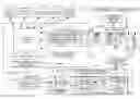

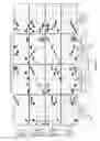
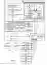
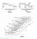
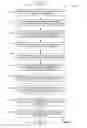
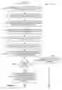
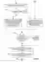
Sources:
- United States Patent and Trademark Office - verify current appl. status at the USPTO↗
Recent applications in this class:
- » 20230254424 2023-08-10
Identification apparatus and image forming apparatus - » 20230188658 2023-06-15
Image forming apparatus, information processing apparatus, information collecting method, and recording medium - » 20220394146 2022-12-08
Identification apparatus, processing apparatus, processing method, and storage medium - » 20220377193 2022-11-24
Information processing apparatus, image forming apparatus, and non-transitory computer readable medium - » 20220210284 2022-06-30
Information processing apparatus and image forming system - » 20210377410 2021-12-02
Image forming apparatus improved in setting process for recording medium, method of controlling the same, and storage medium - » 20210297543 2021-09-23
Image reading device, medium conveyance device, and image forming apparatus - » 20210067647 2021-03-04
IMAGE FORMING APPARATUS AND PROGRAM - » 20200259970 2020-08-13
Image forming apparatus - » 20190373124 2019-12-05
Image forming apparatus, condition determination method, and computer program