Multi-source Pumping Optimization

Description

CROSS-REFERENCE TO RELATED APPLICATIONS

Not Applicable

STATEMENT REGARDING FEDERALLY SPONSORED RESEARCH OR DEVELOPMENT

Not Applicable

REFERENCE TO SEQUENCE LISTING, A TABLE, OR A COMPUTER LISTING COMPACT DISC APPENDIX

Not Applicable

BACKGROUND OF INVENTION

It wasn't long ago that water/wastewater utilities believed that energy efficiency was simply a cost of doing business. The cost of energy was embedded into the price of the product or service and passed along to the customer. Today, however, faced with constrained revenues combined with increasing costs, managers are being forced to take a hard look at ways to either increase revenues or reduce expenses. As you can imagine, increasing rates or reducing jobs are not very popular alternatives. However, one area that can certainly help the realities of this economic outlook is the potential expense reduction in energy consumption, generally a water/wastewater facility's second highest operating expense.

Water/wastewater is an energy-intensive operation. There are in excess of 75,000 water and wastewater systems in the United States alone, estimated to consume well over 150 billion kilowatt-hours (kWh) a year, approximately 12% of the total electricity consumed in the non-residential, commercial and industrial sectors. And if consumption growth is in line with overall energy projections, this will increase by 29% by 2040 (U.S. Energy Information Administration), further adding to the economic challenges water/wastewater providers face today.

The majority of water processing and distribution energy consumption is by motors and motor-driven systems related to pumping. Given that over 80% of the electricity used by water systems is from pumping, most of the energy reduction gains can be realized through operating the water pump systems more efficiently. These efficiencies are gained not only from a design and asset life-cycle management perspective, but by operating the right (most efficient available) pump(s), at the right time, for the right duration, to meet operational requirements at the least cost.

To ensure availability for a specific process, most water operations have built-in pump system redundancy to satisfy operational availability and capacity requirements. Each pump system supporting a specific pump process may be common in design purpose; however, they are typically unique due to disparate operating efficiency. Pump system efficiency can vary greatly depending on the age, design, and operation and maintenance of the system over time. Couple this with the fact that the cost to operate a pump system is dependent on time-of-use (T-O-U) and electricity rates (peak rates can vary by more than 500% from normal and off peak rates), systems availability, and varying demand, it's evident that operating multi-source pump systems for optimum performance at the least energy cost is a complex operational problem.

Optimal multi-source pump system performance at the least energy cost must factor in the pump process system design (what specific pump systems comprise what unique pump process), and each pump system's efficiency, availability, and capacity, and time-of-use energy and demand rates, demand required, and operating strategy (e.g. “peak shaving”, “base load”, and “peak demand avoidance”).

Without the requisite process intelligence, the probability of operating a pumping process at the least cost is not determinable. Access to the intelligence holds significant potential to reduce energy costs.

BRIEF SUMMARY OF THE INVENTION

Patent protection is being requested for a process invention enabled by a web-based software application, (the “Motors@Work System”). The process has been developed to solve the problem of optimizing the operating configuration of a multi-source pumping process. The objective of the Multi-source Pumping Optimization process is to operate the right pumps at the right time to ensure that the required demand is adequately provided by the available pumping system(s) while minimizing the operation cost (energy cost). The decision variables are the operating configuration of the pumping process, the operational time and demand delivered production units of each pump system within a given time frame, and the specific time(s) at which a pumping system operates within the given time frame. A mixed efficiency and optimization coding methodology is developed according to the characteristics of the decision variables.

The Multi-source Pumping Optimization process capability described will answer the following:

• • Which pump system(s) should be operating to meet daily demand
  • How long should each pump system operates per day
  • When should each pump system operate per day
  • What is the pump system delivered production units and operating cost per unit, per hr., per day
  • What is it costing to operate the pump process per day
  • Are there opportunities to reduce Utility demand charges
  • Are there opportunities to reduce Utility peak rate usage charges

It is estimated that daily pumping process operation cost savings of approximately 10% to 25% are attainable by application of the process described within this non-provisional patent application for the Multi-source Pumping Optimization process.

BRIEF DESCRIPTION OF THE SEVERAL VIEWS OF THE DRAWING

FIG. 1.0—Calculating Pump System Efficiency Flow Chart FIG. 1.0 illustrates how a user selects a specific available component pump system in a pumping process, and then calculates the pump system energy profile taking into consideration the system's pump systems component specifications and readings, and then calculates the pump system energy efficiency.

FIG. 2.0—Optimizing Pump Schedule Flow Chart FIG. 2.0 illustrates a User selects a specific pumping process, selects available pump system(s) in that pumping process and then optimizes the use of the selected pump system(s), taking into consideration the T-O-U utility rates, capacity needed for a specific time period, demand charges, operating strategy (e.g. “peak shaving”, “base load”, and “peak demand avoidance”), and selected pump system(s) motor energy efficiencies and capacity.

FIG. 3.0—Minimal Nominal Efficiency Table FIG. 3.0 specifies the motor efficiency by horse power, synchronous speed, enclosure type and efficiency class.

DETAILED DESCRIPTION OF THE INVENTION

Definitions

The definitions of terms pertaining to the Detailed Description of the Invention are defined below.

• • Base load—demand production required on a continual basis during scheduling time frame
  • Capacity—quantity capable to produce
  • Demand—production unit capacity (MGD) required for a pump process
  • Demand charge—Charge for maximum instantaneous energy demand
  • Efficiency—the ratio of usable power to electric input power
  • Flow rate—rate (MGD) at which water is processed to meet demand.
  • HP—Horse power of a motor
  • kW—kilowatt; a measure of electrical power equivalent to 1,000 watts
  • kWh—a unit of energy equivalent to one kilowatt (1 kW) of power consumed for one hour.
  • Peak Demand—the maximum instantaneous demand of electricity in a Utility

Billing Cycle.

• • Peak shaving—the process of shifting demand from peak usage times (“Peak T-O-U Rates”) to times with lower demand (“Off-Peak T-O-U Rates”)
  • Pi (π)—a mathematical constant, the ratio of a circle's circumference to its diameter, commonly approximated as 3.14159.
  • PSI—pounds per square inch
  • Motors@Work System (hereafter referred to as “the System”)—a web based motor management system and multi-source Pump operations configurator
  • Motor—a machine powered by electricity that supplies motive power to a pump
  • MGD—Million Gallons per Day
  • Pump—a device, driven by a motor, for moving water from one place to another by means of a set of rotating vanes
  • Pumping Process—a specific process comprised of 1 or many pump systems, with the objective of moving water from one place to another.
  • Pump System—a system comprised of a motor, pump, and piping components
  • Time-of-Use (T-O-U) Rate—variable Utility Rate pricing based on time-of-use of electricity by the consumer. Rates are typically categorized by “Peak”, “Off-peak”, “Normal”, “Weekend”, “Weekday”, and “Time-of-year”. T-O-U rates are intended to help control peak loads and reduce need for new generation capacity.
  • RPM—Revolutions per Minutes
  • UOM—Unit of Measure
  • VFD—Variable Frequency Drive

INTRODUCTION

The invention, the Multi-source Pumping Optimization process, will determine an optimized pump system schedule for a pumping process. The Multi-source Pumping Optimization process will also determine the schedule's associated delivered production units (MGD), demand (kW), cost (energy consumption and peak demand), and non-conformance intelligence (i.e. projected peak demand, demand not met, and each specific pump system(s)' piping efficiency, hydraulic efficiency, demand kW, and motor load).

The Multi-source Pumping Optimization process is a two-step process. The first step (Calculating Pump System efficiency) determines the efficiency of each pump system based on the pump system's motor, piping and hydraulic efficiencies. The second step (Optimizing Pump Schedule) determines the optimized pump process schedule based on the component pump system(s) availability, efficiency, and capacity, and operating and energy management strategies, combined with the electricity T-O-U tariff and the demand requirements.

The Multi-source Pumping Optimization process being described assumes the following for the selected pump process to be optimized:

• • Pumping process is selected
  • Pump system(s) available to the process are identified
  • Pump system specification is defined (pump(s); motor(s); piping specification(s))
  • Pump capacity is defined
  • Utility rate data is defined
  • Pump system motor efficiency is determined
  • Pump system efficiency is determined
  • Demand required is known
  • Operating and energy management strategies are defined

Ultimately the process will enable the user to select a pump process, select relevant pump system(s) in that pump process and then the Motors@Work System will automatically optimize cost taking into consideration the utility T-O-U rates and demand charges, and User defined constraints.

Process Description

1.0 Calculating Pump System Efficiency

The Pump System Efficiency Calculation (Step 1) process specifications are described below. The paragraph numbers correspond to the process step's reference numbers on Drawings: FIG. 1.0—Calculating Pump System Efficiency Flow Chart.

1.1 Capture Motor Nameplate Information

In order to calculate the electrical motor efficiency, some characteristics of the motor must be known. These characteristics will be available on the nameplate attached to the motor or in the motor's documentation.

Required Motor Data (nameplate):

• • Size (HP)
  • Synchronous Speed (RPM)
  • Enclosure Type
  • Full Load Efficiency (%)

Some data is optional. Different methods may be used to calculate the motor's operating efficiency (below) depending on which data is known/available.

Optional Motor Data:

• • Full Load Amps
  • Wired For Voltage
  • Full Load Speed

1.2 Capture Motor Energy Readings

Using a multi-meter, sub-meter, or other device for obtaining electric readings, gather the following data for each motor.

• • Voltage AB
  • Voltage BC
  • Voltage CA
  • Current A
  • Current B
  • Current C
  • Power Factor
  • Measured Speed
  • Power Draw

1.3 Calculate Motor Energy Profile

Using motor nameplate data and the energy readings taken from the motor, the System calculates motor load and efficiency.

To calculate load; if a Power Draw measurement is entered in the System and the motor Size and Full Load Efficiency are filled in the System then:

Field	Value
Motor Load	Power   Draw ( Size * 0.746 / ( Full   Load   Efficiency 100 ) ) * 100
	Assumptions:
	Power Draw is recorded as kW.
	Size is in HP. If Size is in kW do not multiply with 0.746).
Load	“kW Ratio − Power based”
Estimation
Method

Else if Voltage (AB, BC, and CA), Current (A, B, and C) and Power Factor measurements are entered in the System and the Motor Size and Full Load Efficiency are filled in the System then:

Field	Value
Motor Load	Average   Voltage * Average   Current * Power   factor 100 * 3 1000 ( Size * 0.746 / ( Full   Load   Efficiency 100 ) ) * 100
	Assumptions:
	1. Size is in HP. If Size is in kW do not multiply with
	0.746).
Load	“kW Ratio − Voltage based”
Estimation
Method

Special considerations for the kW Ratio method only:

• • If the Full Load Efficiency of the motor is not entered the System will use the Full Load Efficiency of the Minimal Nominal Efficiency Table (Drawings: FIG. 3.0—Minimal Nominal Efficiency Table). See below section; the System calculates the motor efficiency as follows.
    Else if Average Voltage and Average Current measurements are entered in the System and the motor Full Load Amps and Wired For Voltage are filled in the System then:

Field	Value
Motor Load	( Average   Current Full   Load   Amps ) * ( Average   Volts Wired   For   Voltage ) * 100
	Assumptions:
	2. All currents are in Amps.
	3. All voltage is in Volts.
Load Estimation	“Voltage Compensated Amps Ratio”
Method

Else if Average Voltage and Measured Speed measurements are entered in the System and the motor Synchronous Speed and Full Load Speed and Wired For Voltage are filled in the System then:

Field	Value
Motor Load	Synchronous   Speed - Measured   Speed ( Synchronous   Speed - Full   Load   Speed ) * ( Wired   For   Voltage Average   Voltage ) ) 2 * 100
	Assumptions:
	1. All speeds are in RPM.
	2. All voltage is in Volts.
Load	“Voltage Compensated Slip”
Estimation
Method

The System calculates the motor efficiency as follows:

• • If Motor Load is not blank in the System then the System will find the full load efficiency and efficiencies at 75%, 50% and 25% load for the motor as follows:
    • Use the motor nameplate efficiency percentages if populated in the System.
    • Or search the Minimal Nominal Efficiency Table (Drawings: FIG. 3.0—Minimal Nominal Efficiency Table) where the Horse Power, Synchronous Speed, Synchronous Speed UOM, Enclosure Type and Efficiency Class are the same as that of the motor nameplate. The search will also include the setting of Wired For Voltage. If equal or less than 600 Volts the efficiency records for the “Low Voltage” Voltage Group will be used, otherwise the system uses the “Medium Voltage” group.
  • If no data is found in the System the Motor Efficiency will be blank in the System

	Field	Value
	Motor Efficiency	Blank

• • If data is found in the System the System will compare the calculated Motor Load with the efficiency percentages and populate two variables (Minimum and Maximum Efficiency) and set the Load base variable as follows:

			Load
Motor Load	Minimum Efficiency	Maximum Efficiency	Base

<=25%	0	Efficiency at 25%	0
		Load
>25% and <=50%	Efficiency at 25%	Efficiency at 50%	25
	Load	Load
>50% and <=75%	Efficiency at 50%	Efficiency at 75%	50
	Load	Load
>75%	Efficiency at 75%	Full load efficiency	75
	Load

• • If the Motor Load is above the 75% threshold the Maximum Efficiency will be replaced with the System's header motor nameplate Full Load Efficiency providing this value is entered in the System and higher than Maximum Efficiency.
  • The System will determine the Slope. Slope is the linear slope between the Minimum and Maximum Efficiency as follows:
    • (Maximum Efficiency−Minimum Efficiency)/25
  • If the Motor Load is greater than 25% then the System will calculate the Motor Efficiency as follows:

	Field	Value
	Motor Efficiency	(Motor Load − Load Base) * Slope +
		Minimum Efficiency

• • Otherwise if the Motor Load is less than or equal to 25% then the System will calculate the Motor Efficiency (=load served/load served plus the fixed losses at 25% of the load) as follows:

Field	Value
Loss at 25%	Size * 0.25 * ( 1 ( Maximum   Efficiency / 100 ) - 1 )
Horse Power at Load	Size * Motor   Load 100
	Note: The Size UOM is not relevant for this calculation.
	Conversion from HP to kW is not required.
Motor Efficiency	Horse   Power   at   Load Horse   Power   at   Load + Loss   at   25  % * 100

• • If the Motor Load was calculated with one of the two kW Ratio techniques the System will recalculate the Motor Load with the calculated Motor Efficiency instead of the Full Load Efficiency and will stay in this loop until either:
    • The difference between two consecutive Motor Loads is less than 0.05 or
    • The System has recalculated 50 times.
  • If Rewound is selected for the System header motor then the calculated Motor Efficiency is corrected as follows:

	Motor Size in HP	Rewound Correction

	<=40	0.5%
	>40	0.25%

	Field	Value
	Motor Efficiency	Motor Efficiency − Rewound Correction

1.4 Capture Pump Nameplate Information and Operations Statistics

Gather the following nameplate data for each pump and enter in the System. The Static Suction Head and Discharge Head data can be attained from drawings or estimates.

• • Inlet Diameter
  • Outlet Diameter
  • Design Friction Losses
  • Length of Discharge Pipe
  • Static Suction Head
  • Static Discharge Head

Capture the following pump operation statistics and enter in the System. The Pump Discharge Pressure can be attained from a pressure gauge, and the flow Pump Discharge Flow Rate data from a flow meter or estimate.

• • Pump Discharge Flow Rate
  • Pump Discharge Pressure
  • Fluid Density
    The System then calculates the Pump System Efficiency.

1.5 Calculate Pump System Energy Profile

The System calculates the Pump System Efficiency as follows. The System calculates Pump System Efficiency performance with the gravitational constant g set at 9.80665 m/s² as follows:

Field	Value
Inlet Velocity (m/s)	Pump   Discharge   Flow   Rate ( π * Pump   Inlet   Diameter 2 4 * 3600 )
Outlet Velocity (m/s)	Pump   Discharge   Flow   Rate ( π * Pump   Outlet   Diameter 2 4 * 3600 )
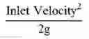
Velocity Head Inlet (m of head)	Inlet   Velocity 2 2   g
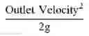
Velocity Head Outlet (m of head)	Outlet   Velocity 2 2   g
Velocity Head	Velocity Head Outlet − Velocity Head Inlet
(m of head)
Total Head	Static Suction Head + Pump Discharge Pressure + Velocity Head
(m of head)
System Friction Losses	Pump Discharge Pressure − Static Discharge Head
(m of head)
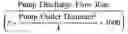
Temp Flow Density	Pump   Discharge   Flow   Rate * Fluid   Density * g 3600000
Pump Discharge Power	Pump Discharge Pressure * Temp Flow Density
(kW)
Static Suction Power (kW)	Static Suction Head * Temp Flow Density
Velocity Head Power (kW)	Velocity Head * Temp Flow Density
Pump Hydraulic Power	Pump Discharge Power + Static Suction Power +
Output (kW)	Velocity Head Power
Motor Power (kW)	Find the Motor Load of the most recent measurement for the
	motor of the pump. Find the Size for this motor. If size specified
	in HP multiply by 0.746 kW/HP to convert size to kW.
	Motor Power = Size * Motor Load / 100
Pump Hydraulic	Pump Hydraulic Power Output / Motor Power * 100
Efficiency (%)
Piping Efficiency (%)	100 - ( Pump   Discharge   Pressure - Static   Discharge   Head ) * 100 Pump   Discharge   Pressure
System Efficiency (%)	Motor Efficiency * Pump Hydraulic Efficiency * Piping
	Efficiency / 10000
Best Achievable Piping Efficiency (%)	100 - ( Length   of   Discharge   Pipe - Design   Friction   Loss ) * 100 Pump   Discharge   Pressure

Note: the System calculates data conversion if necessary as follows:

Field	Value
Pump Inlet Diameter	See below in Table 1; Convert Length.
Pump Outlet Diameter	See below in Table 1; Convert Length.
Pump Discharge Flow Rate	See below in Table 2; Convert Flow Rate.
Static Suction Head	See below in Table 1; Convert Length.
Static Discharge Head	See below in Table 1; Convert Length.
Pump Discharge Pressure	See below in Table 3; Convert Pressure.
Fluid Density	See below in Table 4; Convert Density.

To convert from one UOM to another the System will:

• • 1. Find the row the represents the From UOM in the following conversion Tables (2, 3, 4 and 5).
  • 2. Divide by the conversion factor found in the cell where the row and column intersect.
    For example, to convert the Inlet Diameter from Feet to Meters divide by 0.30483

	TABLE 2
	Convert Length	Conversion factor to Meters

	From Meters	1
	From Centimeters	100
	From Feet	3.28084
	From Inches	39.37008

TABLE 3
Convert Flow Rate	Conversion factor to Cubic Meters/Hour

From Cubic Meters/Hour	1
From Imperial Gallons/Hour	219.969
From US Gallons/Hour	264.172
From Cubic Meters/Minute	From Cubic Meters/Hour/60
From Imperial Gallons/Minute	From Imperial Gallons/Hour/60
From US Gallons/Minute	From US Gallons/Hour/60

	TABLE 4
	Convert Pressure	Conversion factor to Meters of Head

	From Meters of Head	1
	From Feet of Head	3.28084
	From Bar	0.098068059
	From PSI	1.421969428

TABLE 5
Convert Density	Conversion factor to Kilogram/Cubic Meter

Kilogram/Cubic Meter	1
US Pound/Cubic Feet	16.01846337

2.0 Optimizing Pump Schedule

The System having completed Calculating Pump System Efficiencies (Step 1) the Optimizing Pump Schedule (Step 2) process (Step 2) is now able to be performed. The Optimizing Pump Schedule process specifications are described below. The paragraph numbers correspond to the process step's reference numbers on Drawings: FIG. 2.0—Optimizing Pump Schedule Flow Chart.

2.1 Select Pump System(s) for Consideration

Choose a pump process in the System to optimize and identify the pump system(s) that are available to participate in the pump process. Select the available pump system(s) for consideration in the System.

2.2 Determine Applicable Utility Rate Structure

Determine the Utility Rate Structure that applies to the day in question including T-O-U and demand charge rates. Enter or select the Utility Rate Structure in the System.

2.3 Determine Required Production by Hour or by Day

Based on operational requirements, historical trends, or experience, estimate how much demand is required for the time period to be optimized. Enter the demand in the System.

2.4 Calculate Cost of Running Pump System by Hour

For each selected pump the System will determine demand kW and demand charge for the day to optimize.

• • Pump System Demand kW=(HP*0.746*Motor Load %)/Motor Efficiency
    • Note: The System will take motor efficiency here only. The other components that make up the pump system efficiency are not relevant since they are already represented in the motor load and the only thing the System is calculating here is the energy consumption of the motor. The System only needs motor load and motor efficiency. The piping and hydraulic efficiency calculations are used to determine potential pump system design efficiency opportunities (i.e. mitigate pumping system motor load).
  • Pump System Demand Charge=Pump System Demand kW*Demand Charge per kW

Next, for each selected pump system the System will determine Cost per Production UOM and Hourly Running Cost for the Day to optimize

• • If Daily Pump System Capacity is not available in the System then the Cost per Production UOM and Hourly Running Cost are both blank.
  • Cost per Production UOM
    • Pump System Energy Usage=(HP*0.746*Motor Load %)/Motor Efficiency. This is then considered a constant for this optimization run.
    • For each hour of the day:
      • Cost Pump System Energy Usage=Pump System Energy Usage*Utility Rate of that hour
      • Cost per Production UOM=Cost Pump System Energy Usage/(Daily Pump Capacity/24)
  • Hourly Running Cost=Pump System Demand kW*Utility Rate of that hour
  • Hourly Pump System Capacity=Daily Pump System Capacity/24
    2.5 The System sorts Pump System Cost List from Lowest Cost to Highest

For each selected pump system and for each day to optimize the System will now have 24 (one per hour) Cost per Production UOM, Hourly Running Cost calculated and the Pump System Hourly Pump Capacity per hour. The System then put each hour for each Pump System into a set of records and sorts these records on a Cost per Production UOM (ascending), then on Priority (ascending) of the Pump System, then on hour (ascending). This leads to the Delivery Matrix. An example Delivery Matrix is provided below.

Example Delivery Matrix:

			Cost per	Hourly			Base
			Produc-	Pump	Hourly		Load
Pump	Rate		tion	Capac-	Running	De-	De-
System	Code	Hour	UOM	ity	Cost	liver	livery

Pump x	Off peak	00	.0123	80	0.984
Pump x	Off peak	01	.0123	80	0.984
		. . .
Pump x	Off peak	08	.0123	80	0.984
Pump x	Off peak	20	.0123	80	0.984
Pump x	Off peak	21	.0123	80	0.984
		. . .
Pump x	Off peak	23	.0123	80	0.984
Pump y	Off peak	00	.09	120	10.8
Pump y	Off peak	01	.09	120	10.8
		. . .
Pump y	Off peak	08	.09	120	10.8
Pump y	Off peak	20	.09	120	10.8
Pump y	Off peak	21	.09	120	10.8
		. . .
Pump y	Off peak	23	.09	120	10.8
Pump x	Peak	09	.134	80	10.72
Pump x	Peak	10	.134	80	10.72
		. . .
Pump x	Peak	19	.134	80	10.72
Pump y	Peak	09	.19	120	22.8
Pump y	Peak	10	.19	120	22.8
		. . .
Pump y	Peak	19	.19	120	22.8

2.6 the System Adds the Next Lowest Cost Pump-Hour to Schedule

With Daily Demand specified, Base Load and Hourly Demand not specified the System will;

• • Loop through the sorted Delivery Matrix from top to bottom, i.e. in the sequence the data is sorted and set Deliver is Hourly Pump Capacity until SUM (Deliver)>=Daily Demand.
  • Correct the last Deliver so that in this sequence:
    • Sum (Deliver)=Daily Demand if the pump system selected has a VFD.
    • Otherwise apply the pump system that has a VFD and that can satisfy the remaining demand with the cheapest Cost per Production UOM.
    • Otherwise minimize the Hourly Running Costs, i.e. apply the pump without a VFD that has the least Hourly Running Cost that can satisfy the remaining demand.

With Hourly Demand specified the System will;

• • If a specific demand is specified for an hour or hours of the day the System behaves as described above under Daily Demand specified, base Load And Hourly Demand Not Specified except the system will satisfy the Hourly Demand by only using the rows in the Delivery Matrix where Hour matches the hour or hours the hourly demand is specified for.

Operations sometimes have a minimum base load that the process must constantly deliver at a minimum. If that is the case, use the following process to identify the optimal pump configuration.

With Base Load Demand requirement

• • The System will determine the base load demand requirement per Hour.
    • Take Hourly Base Load Demand if specified for that hour
    • If not specified take the Daily Base Load Demand and
      • Subtract the SUM of all specified Hourly Base Load Demand for that day.
      • Divide the difference by the number of hours on that day that do not have an Hourly Base Load Demand specified.
        • If the difference is <zero set it to zero, i.e. the individual Hourly Base Load Demand together add up to more than the Daily Base Load Demand and hence the Daily Base Load is already covered.
        • The System will not divide by zero. If there are no hours without an Hourly Base Load Demand then Hourly Base Load Demand will be used and the Daily Base Load Demand will be ignored. The System will set the difference to zero.
  • Loop through all hours and assign Pump System(s) to cover the Base Load for that hour. The System behaves similar as described above under; Daily Demand specified, Base Load and Hourly Demand Not specified except the System will assume that every Hour has a specified Demand and that Demand is equal to the Base Load.
  • In the Delivery Matrix all Pump System(s) assigned to Base Load delivery will be flagged as Base Load Delivery. The System will assign the Delivered Capacity to the Base Load Delivery Column.
  • The System will then loop through the hours of the day again as if no Base Load Demand was specified. The System behaves as described above under; Daily Demand specified, Base Load and Hourly Demand Not Specified and with Hourly Demand Specified.
  • The System now verifies superfluous delivery. Hours that have a Base Load Delivery but no or less Delivery add to the total Delivery and hence increase total Delivery and therefore total Delivery may now exceed Daily Demand. This is ONLY possible for the hours where no specific Hourly Demand was specified. As follows:
    • Determine SUM (Delivery for all hours without specific Hourly Demand)
    • Loop through the Delivery Matrix but now in sequence of the Cost per Production UOM (descending), then on Priority (descending), then on Hour (descending) only selecting records where Delivery>zero.
    • The System will switch off Pump System (set Delivery=blank) as long as SUM (Delivery for all hours without specific Hourly Demand)>Daily Demand minus SUM (all specific Hourly Demand for that day). The System will only switch off Pump Systems where Base Load Delivery=blank.

Example Delivery Matrix for 750 Gallons:

Pump			Cost per	Capacity
System	Rate Code	Hour	Production UOM	Per Hour	Deliver

Pump x	Off peak	00	.0123	80	80
Pump x	Off peak	01 . . .	.0123	80	80
Pump x	Off peak	08	.0123	80	80
Pump x	Off peak	20	.0123	80	80
Pump x	Off peak	21 . . .	.0123	80	80
Pump x	Off peak	23	.0123	80	80
Pump y	Off peak	00	.09	120	120
Pump y	Off peak	01	.09	120	120
Pump y	Off peak	02	.09	120	30
Pump y	Off peak	03 . . .	.09	120
Pump y	Off peak	8	.09	120
Pump y	Off peak	20	.09	120
Pump y	Off peak	21 . . .	.09	120
Pump y	Off peak	23	.09	120
Pump x	Peak	09	.134	80
Pump x	Peak	10 . . .	.134	80
Pump x	Peak	19	.134	80
Pump y	Peak	09	.19	120
Pump y	Peak	10 . . .	.19	120
Pump y	Peak	19	.19	120

2.7 Determine the Cost for Each Entry Delivered in the Delivery Matrix

Now that the System Delivery Matrix is complete the system will determine Costs. For each Pump System running it is determined how much this Pump System costs and what the total for all Pump System are.

• • Additional Cost column in the Delivery Matrix.
  • Every row in the Delivery Matrix gets a Cost associated. Cost is Deliver*Cost per Production UOM.
    • Note: This is mostly the same as the original Cost Pump System Energy Usage, but if Deliver is less than the Pump System Capacity, i.e. the Pump System does not run the full hour, it will be less.

			Cost per Production
Pump	. . .	Hour	UOM	Deliver	Cost
Pump x	. . .	00	.0123	80	0.984
Pump x	. . .	01 . . .	.0123	80	0.984
. . .

2.8 Avoid Peak Demand Charges

At this point the System has determined a Delivery Matrix for each Day to Optimize that uses as many Pump Systems as required to minimize the Pump Process operational costs. The System will use more Pump Systems at off peak rates. More Pump Systems operating concurrently however means a higher Peak Demand which translates to higher Utility bills due to higher Peak Demand charges levied by the Utility. The System optimization process will determine if Peak Demand charges can be avoided. The System inputs required are:

• • Remaining days in the Utility Billing Cycle. By entering the date of the last bill in the System the System will determine this by determining the remaining days from the current day assuming that the current month bill will occur on the same day as the previous month. This date is stored and retrieved as long as required, until changed by the user. If the last bill is not entered into the System the System will simply assume a calendar month.
  • Period Peak Demand of this billing cycle. As long as the System stays below the established Period Peak Demand the System is not increasing costs for this billing cycle. The System Period Peak Demand value may be related to a future day in the billing cycle. The System keeps track of this in Current Month Projected Peak Demand (kW).
  • Incurred Period Peak Demand. The actual Peak Demand in the billing cycle. The System keeps track of this in Current Month Actual Peak Demand (kW).
    • Note: If metered (Measured Peak) the System store this and use this actual measured value. This value must have occurred in the past. It is an actual historical value.

The System now verifies if this step is necessary, i.e. Avoid Demand Peak (kW) is selected, and if it is starts a loop in which it tries to reduce the peak demand for each day to optimize, as follows:

• • Determine Peak Demand=SUM (Pump System Energy Usage for each distinct Pump System in the Delivery Matrix). The System determines this for every hour in the matrix and takes the highest number (not all Pump Systems are running all the time).
    • Convert Peak Demand and Period Peak Demand to a monetary value by multiplying with the Demand Charge. Demand Charge may be different per day. The System will pick relevant Demand Charge automatically.
  • Compare this with the current Period Peak Demand for this billing cycle. The System will use the monetary values for this comparison. If Peak Demand<Period Peak Demand then:
    • The System will skip this step of the Peak Demand Charge Avoidance process for this Day to Optimize.
    • Otherwise the System will continue with the next steps and try to reduce peak demand.
  • For the Day to Optimize the System will find the last Pump System that was added to the Delivery Matrix. The last Pump System is also the most expensive pump (Cost per Production UOM) of all that are included in the Delivery Matrix and therefore it makes sense for the System to first try and remove that from the Delivery Matrix.
  • Determine the Pump System Demand Charge for this Pump System
    • Pump System Demand Charge=Pump System Energy Usage*Demand Charge per kW.
    • The System spreads this charge over the remaining days in the billing cycle, i.e. Daily Pump System Demand Charge=Pump System Demand Charge/Remaining Days.
      • Note: If the optimization includes more days than fit in the billing cycle the System will use the numbers from the respective billing cycle.
    • Determine Total Delivery to Avoid. This variable is equal to the SUM (Delivery) for this Pump System. The System adds up all Delivery for all rate codes, since there may be more. For example in the Delivery Matrix below this is 270 for Pump System Py.
    • The System will go to the first Pump System (ascending) in the Delivery Matrix that has hours available.
      • Fills the empty hours with the Delivery for that Pump System.
      • Subtracts added Delivery from Total Delivery to Avoid.
      • Continues performing this process until Total Delivery to Avoid is 0
      • If the first Pump System has no capacity left the System will proceed to the next and repeat until complete or the selected Pump Systems run out of capacity.
        • Important: The Delivery Matrix is still sorted. Assigning capacity must follow this sequence. This means that in a scenario where there is three Pump Systems (x which is the cheapest, y and z which is the most expensive) and there are three rate codes the Delivery Matrix will show x,y,z for the low rate, x,y,z for the intermediate rate and x,y,z for the high rate. So if the System is trying to remove z and the System had only used the low rate this process the System will reassign in sequence x,y the intermediate rate and then x,y the high rate.
      • If the selected Pump Systems run out of capacity, meaning there are not enough available hours in the Delivery Matrix to offset Total Delivery to Avoid, then the System will indicate this (Optimization Alert) to the user. This is only necessary if the first Pump System could not be removed from the peak. The second or a later Pump System will ultimately run into this constraint and this is acceptable at that time.
      • The System now calculates the costs (Delivery*Cost per Production UOM) of this reassignment.
      • The System compare the costs of Daily Pump System Demand Charge+Cost of running the Last Pump System with the costs of the extra Delivery by the first Pump System and any consecutive Pump Systems needed to cover for the last Pump System. The latter would normally be higher costs per unit since the System is now using the higher rates for these (off peak or low rates are already used up). If favorable (costs of the extra Delivery of the first and consecutive pumps is less) the System will remove the last Pump System and apply the Delivery required to replace the last Pump System to the first and consecutive Pump Systems as calculated.
    • The System will repeat with the now new last Pump System until there is no capacity left.
  • When the Peak Demand Avoidance loop is finished or in case the step was skipped the System will calculate Peak Demand for the Day to Optimize=SUM (Pump Energy Usage for each distinct Pump System in the Delivery Matrix). The System will do this for every hour in the matrix and take the highest number (not all Pump Systems are running all the time).
    • Note: Convert to monetary value.
  • This value will be stored for this Day to Optimize.
  • Determine Incurred Period Peak Demand for past days, i.e. the System finds the highest Peak Demand for yesterday and the days before yesterday, but stays within the billing period.
  • If Peak Demand for the Day to Optimize>Period Peak Demand for this billing cycle the System will set:
    • Period Peak Demand for this billing cycle equal to Peak Demand of the Day to Optimize.
  • Else if the Day to Optimize is today or a future date in the current billing cycle then if Peak Demand for Day to Optimize<Period Peak Demand for this billing cycle, then it is possible that this day (the Day to Optimize) actually caused the previous peak for the billing cycle. Therefore the System must verify this and possibly reset the peak to the lower, but currently highest, peak value as follows:
    • Set Period Peak Demand for this billing cycle equal the highest value for Peak Demand found for the remaining days in the billing cycle starting at the current System Date. Compare this with the Incurred Period Peak Demand and set Period Peak Demand equal to the highest value.
    • However, if Day to Optimize is for a future billing cycle, then the System will take all days in that future billing cycle.
  • The System displays the
    • Incurred Period Peak Demand in Current Month Actual Peak Demand (kW)
    • and Period Peak Demand in Current Month Projected Peak Demand (kW)
    • Both of these values are multiplied with the Demand Rate (monetary value).
      Delivery Matrix per pump/hour before peak demand charge avoidance:

Pump	0	1	2	3	4	5	6	7	8	9 thru 19	20	21	22	23

Px	80	80	80	80	80	80	80	80	80		80	80	80	80
Py	120	120	30

And after:

														13 thru
Pump	0	1	2	3	4	5	6	7	8	9	10	11	12	19	20	21	22	23
Px	80	80	80	80	80	80	80	80	80	80	80	80	30		80	80	80	80
Py

2.9 Peak Shaving

To use the practice of “peak shaving” on the results:

• • If a Base Load is required the System will satisfy the Base Load requirement as usual. All Rate Codes will be used.
  • After the Base Load is scheduled or in case no Base Load is required, then the System will not schedule any Pumps on any rows in the Delivery Matrix where the Rate Code matches the Rate Code identified on the peak shaving scenario or, if the Rate Code is automatically selected, where the Rate Code represents the highest rate ($/kWh).

The Multi-source Pump System Optimization distinctly claims the following subject matter as innovation and invention specific to the multi-source Pump optimization process and configuration tool.