System for determining the position of the position indicator of a position measuring system
US20180080796A1
2018-03-22
15/694,798
2017-09-03
✅ Patent granted
US 10,557,722 B2
2020-02-11
-
-
Mischita L Henson
CanaanLaw, P.C. | David B. Ritchie
2037-09-03
Abstract:
The invention concerns a method for determining a position φ of a position indicator of a position measuring system, in which the sensor signals a1 to ar of a number of r sensors are recorded as a signal vector {right arrow over (a)}=(a1, . . . , ar), a measurement vector {right arrow over (q)} is formed according to {right arrow over (q)}=g({right arrow over (a)}), a 2-component vector {right arrow over (p)} is calculated according to {right arrow over (p)}=M·{right arrow over (q)}, wherein M is a 2×n matrix, and the position φ is determined by means of a predetermined function ƒ({right arrow over (p)}) to φ=ƒ({right arrow over (p)}), wherein the function ƒ({right arrow over (p)})=ƒ(p1,p2) is based on the equations p1=cos(φ) and p2=sin(φ). The matrix M is determined in a calibration phase in such a manner, that the transformation {right arrow over (p)}=M·{right arrow over (q)} is a linear mapping, which maps a number m of measurement vectors {right arrow over (q)}k on 2-component vectors {right arrow over (p)}k, wherein the tips of the vectors {right arrow over (p)}k substantially lie on a circle or on a circular arc. The method allows the elimination of external fields.
Assignee:
- NM Numerical Modelling GmbH 1 🇨🇭 , Switzerland
- maglab AG 2 🇨🇭 , Switzerland
Applicant:
Interested in similar patents?
Get notified when new applications in this technology area are published.
Classification:
G01D5/14 » CPC main
Mechanical means for transferring the output of a sensing member; Means for converting the output of a sensing member to another variable where the form or nature of the sensing member does not constrain the means for converting; Transducers not specially adapted for a specific variable using electric or magnetic means influencing the magnitude of a current or voltage
G01D5/244 IPC
Mechanical means for transferring the output of a sensing member; Means for converting the output of a sensing member to another variable where the form or nature of the sensing member does not constrain the means for converting; Transducers not specially adapted for a specific variable using electric or magnetic means influencing characteristics of pulses or pulse trains; generating pulses or pulse trains
H02K11/215 » CPC further
Structural association of dynamo-electric machines with electric components or with devices for shielding, monitoring or protection for measuring, monitoring, testing, protecting or switching; Devices for sensing speed or position, or actuated thereby Magnetic effect devices, e.g. Hall-effect or magneto-resistive elements
G01D5/145 » CPC further
Mechanical means for transferring the output of a sensing member; Means for converting the output of a sensing member to another variable where the form or nature of the sensing member does not constrain the means for converting; Transducers not specially adapted for a specific variable using electric or magnetic means influencing the magnitude of a current or voltage using Hall-effect devices influenced by the relative movement between the Hall device and magnetic fields
G01D5/24476 » CPC further
Mechanical means for transferring the output of a sensing member; Means for converting the output of a sensing member to another variable where the form or nature of the sensing member does not constrain the means for converting; Transducers not specially adapted for a specific variable using electric or magnetic means influencing characteristics of pulses or pulse trains; generating pulses or pulse trains; Error correction Signal processing
H02P6/16 » CPC further
Arrangements for controlling synchronous motors or other dynamo-electric motors using electronic commutation dependent on the rotor position; Electronic commutators therefor; Electronic commutators Circuit arrangements for detecting position
Description
PRIORITY CLAIM
Applicant hereby claims foreign priority under 35 U.S.C § 119 from Swiss Patent Application No. 01207/16 filed on Sep. 16, 2016 and from European Patent Application No. 17167135.7 filed on Apr. 19, 2017, the disclosures of which are herein incorporated by reference.
FIELD OF THE INVENTION
The invention concerns methods for determining the position of the position indicator of a position measuring system, in particular a method for determining the position of a position indicator of a linear position measuring system or of the position indicator of an angle measurement system.
BACKGROUND OF THE INVENTION
Various sensor systems for measuring the position φ of a rotating or linearly moving position indicator are known, in which the information to be obtained is represented by sine and cosine shaped varying raw signals p1=cos(φ) and p2=sin(φ). Possible implementations include e.g. the measurement of components of the induction field of a permanent magnet at suitable locations in space. The searched position is then determined from p1, p2 e.g. via the function φ=a tan 2(p2,p1) by means of the function a tan 2 known from the C-programming language. These prerequisites severely restrict possible arrangements of sensor elements and position indicator, and in particular require a high degree of accuracy in their production or the relative positioning of the sensor chip and the position indicator, respectively.
A fundamental difficulty with these methods is that a non-ideal arrangement of the position indicator and the sensor chip leads to distortions of the raw signals, in particular that these no longer have the pure sine and cosine shape and thus lead to an inaccurate determination of the position φ. There exist methods to improve the raw signal quality, e.g. by using offset and amplitude corrections. A method for a sensor arrangement with two sensors known from WO 2005124286 is based on a description of the measuring points as ellipses and requires specific calibration measurements, which provide parameters for the corrections and which can be realized in practice only with considerable effort. This method requires great care in the design of the sensor arrangement and especially in the adjustment of the permanent magnet, so that the measured values lie sufficiently precisely on an ellipse. If the actual rotational axis does not pass through the magnetically defined center of the permanent magnet, the correction can even cause the opposite effect of an increase in the angular error.
In many instances, a position sensing system is responsive to external fields (e.g., the earth's magnetic field in the case of a position indicator based on permanent magnets). Without countermeasures, these additional field components cannot be distinguished from the useful field so that the external fields restrict the accuracy of the position measuring system.
A fundamental challenge for position measuring systems is their long-term stability, i.e., an initially sufficiently accurate calibration changes over time, e.g. by mechanical displacement of the components relative to one another or by drifting of electronic sensor properties. However, the measurement quality of systems during normal operation is not ascertainable according to the state of the art, in particular this cannot take place intrinsically, i.e. without reference measurements from outside. However, an intrinsic method would be of great importance for fault-tolerant systems. In addition, a recalibration of a position measuring system during normal operation would be very valuable in order to decisively improve the long-term stability.
SUMMARY OF THE INVENTION
The method according to the invention for determining the position of a position indicator is based on the finding that the sensor measurement values supplied by the sensors can be represented as a measurement vector, i.e. as a point in a vector space, the dimension of which corresponds to the number of sensors, and that the measurement vectors generated during the movement of the position indicator (rotation about an axis of rotation or displacement along an axis) lie on a path called orbit in this vector space.
This orbit can—under ideal conditions—be projected onto a circle or a circular arc by means of a linear mapping, i.e. each position of the position indicator corresponds to a point on the orbit in the abstract space of the signal vectors which is unambiguously assigned to a point on the circle or arc. Non-ideal conditions, for example non-ideal properties of the position indicator, which can be particularly the case with magnets, or an insufficient number of sensors or the use of non-optimally selected calibration positions, cause deviations from the circular shape. The linear mapping can be represented as a matrix-vector operation and can be determined using standard methods of linear algebra. Each measurement vector is projected onto a 2-component vector, the tip of which approximates a circular arc, wherein the direction of the 2-component vector corresponds to the position of the position indicator. The linear mapping is determined in a calibration phase, which includes the detection of measurement vectors and the decomposition of a matrix formed by the measurement vectors into two or typically three matrices. The representation of the measured values provided by the sensors as a vector also makes it possible to reduce the influence of external fields, in particular magnetic external fields, by means of a further linear mapping.
The method according to the invention can be used universally. The arrangement of the sensors is virtually arbitrary. The sensors may even detect different components of the field generated by the position indicator. The determination of the matrix can be carried out using measurements which only have to fulfill an absolute minimum of prerequisites. The method is particularly effective without a plurality of angular reference measurements, except the determination of the zero position, which however requires only a single reference measurement. These minimum requirements for the measurements needed for the calibration allow inter alia that a recalibration of the position measuring system is possible during normal operation, or that a factory-based, initial calibration for a given position measuring system can be iteratively improved by means of a bootstrapping method.
Further, in implementations which provide redundant information to the position of the position indicator (e.g., because more than the minimum number of single sensors is installed), one or more of the following additional tasks can be solved:
-
- error detection, i.e. intrinsically detecting a drift and triggering a predetermined action, for example, a corresponding warning or recalibration.
- external field compensation by suppressing external field influences on the measuring signals.
- elimination of errors caused by an offset between the actual axis of rotation of the position indicator and the ideal axis of rotation.
- elimination of errors caused by irregularities of the magnet when the position indicator is a magnet.
- improvement of the signal-to-noise ratio if more than two sensors are used, since then a plurality of individual sensor values enter into the determination of the position and thus an averaging takes place. In particular, difficulties during the zero crossing of the sine or cosine signal of conventional systems can be avoided.
Furthermore, the method for determining the position of a position indicator according to the invention can be designed such that a number of r=2+b sensors are used, and that a projection matrix is used to project the influence of a number of b different external field configurations out of the signal vectors, wherein the projection matrix simultaneously produces 2-component vectors whose tips lie essentially on a circle or circular arc.
BRIEF DESCRIPTION OF THE DRAWING FIGURES
The accompanying drawings, which are incorporated into and constitute a part of this specification, illustrate one or more embodiments of the present invention and, together with the detailed description, serve to explain the principles and implementations of the invention. The figures are drawn schematically and not to scale. In the drawings:
FIG. 1 shows an angle measurement system,
FIG. 2 shows a linear position measuring system,
FIG. 3 shows a resolver, and
FIGS. 4 to 10 illustrate various aspects of the method according to the invention.
DETAILED DESCRIPTION OF THE INVENTION
FIG. 1 shows a position measuring system which has a magnet 2 rotatable about a predetermined axis of rotation 1 and a sensor chip 3. The rotational position of the magnet 2 is the position φ to be determined by means of the sensor chip 3. The sensor chip 3 is shown enlarged on the right-hand side of FIG. 1. The sensor chip 3 comprises a predetermined number of 1 to r sensors 4 and electronic circuits for the operation of the sensors 4, etc. The sensors 4 are, for example, Hall sensors. Such a sensor 4 can also be a cluster of several individual sensors which provide a common output signal. The sensor chip 3 can also contain magnetic field concentrators, which amplify the magnetic field generated by the magnet 2 at the locations of the sensors 4. The number r of the sensors 4 is at least r=2. The sensors 4 each output a sensor signal. The sensor signals are designated herein as a1 to ar. The index j of the sensor signal aj therefore designates the number of the respective sensor 4.
FIG. 2 shows a position measuring system constituted by a magnet 2 and a sensor chip 3 which are displaceable relative to one another along a linear axis x. The sensor chip 3 comprises a predetermined number of 1 to r sensors 4 and electronic circuits for the operation of the sensors 4, etc. The sensors 4 are, for example, Hall sensors. The magnet 2 consists of alternately oppositely magnetized regions which produce a periodically changing magnetic field at the locations of the sensors 4 during a displacement along the axis x. Die x-position of the magnet 2 is the position φ to be determined by means of the sensor chip 3. It is x=D/2π·φ, wherein D is a distance defined by the magnet 2.
The sensors 4 of these position measuring systems provide, as a result of the periodically changing magnetic field, harmonic output signals. The position measuring system of FIG. 1 is an angle measuring system with the rotatable magnet 2 as a position indicator. The position measuring system of FIG. 2 is a linear measuring system with the displaceable magnet 2 as a position indicator. In both position measuring systems, the range of values of the position φ extends over a range from 0 to 2π, which corresponds either to the angular range from 0 to 360° or to a linear range of 0 to D, wherein the distance D results from the fact, that for all j=1, . . . , r sensor signals aj is aj(x+D)=aj(x).
FIG. 3 shows a position measuring system, which is formed from a rotor coil R and from the stator coils Si, i=1, . . . , r with r≧2. The rotor coil R is rotatable about an axis of rotation and is fed with a sinusoidal current which generates a magnetic field. The magnetic field induces in the stator coils Si, i=1, . . . , r a voltage whose amplitude is modulated as a function of the rotational angle r of the rotor coil R. By means of demodulation, sensor signals ai(t), i=1 . . . , r, which vary harmonically with the angle of rotation φ, are generated from the stator coil signals, from which the instantaneous rotational angular position φ(t) of the rotor coil R can be calculated. The signal vector ai(t) consists of the envelope of the signal of the stator coil Si for all i=1, . . . , r.
Position measuring systems can also be based on the inductive principle, in which at least one transmitting coil and at least one receiving coil are spatially fixed, and the position indicator is a geometrically structured, electrically conductive disk which is rotatable about an axis. It is also possible to use the same coil for the transmission and the reception process. The coils can be arranged and/or connected to one another on several levels. The position measuring system can have two or more coils. The use of several coils is particularly helpful to detect the full 360° rotation. The position indicator changes the inductance of the transmitting coil and the receiving coil(s). The transmitting coils are fed with alternating currents, preferably sinusoidal currents, whereby the magnetic fields generate induction voltages in the receiving coils which because of the position-dependent eddy currents generated in the disk have harmonically varying amplitudes. By means of demodulation, the signals for the method according to the invention for determining the position of the position indicator are obtained.
The method according to the invention can also be used in optical position measuring systems in which two or more optical sensors (e.g. phototransistors, photodiodes, etc.) detect in dependence of the position of an optically active position indicator the brightness, polarization, phase shift, time of flight or other optical property variations. For this purpose, the position indicator reflects or modulates a light beam and thus causes the harmonic signals used by the method. Instead of the optical field, such a position meter can also be equipped with radar or terahertz radiation sensors, or corresponding position indicators. In addition, sound waves, in particular ultrasound can also be used instead of optical and electromagnetic waves, and a corresponding position measuring system can be constructed.
The method according to the invention can also be used in electrostatic position measuring systems in which a rotatably mounted geometrically structured electrode as position indicator together with stator electrodes forms two or more capacitors with position-dependent capacitances. Capacitive signals that vary with the position are generated and detected. In an electrostatic system, the position indicator can also be realized by a structured dielectric material which modulates the capacitance of two or more spatially fixed electrode pairs harmonically with the position.
The method according to the invention also makes it possible to separate the useful signal or the useful signals from interfering signals. An example is a magnetic rotary encoder on an electric motor. In this case, the magnetic field of the magnetic angle sensor can be separated cleanly from the rotating fields of the electric motor. Thus, the position can be determined without interference. This also applies to optical, electro-magnetic, electrical, magnetic, and acoustic position determinations.
All these physical principles can be used both for the construction of a position measuring system with a rotatably mounted position indicator as well as with a linearly displaceably mounted position indicator.
The invention relates to a method by which the position φ can be calculated from the measured values delivered by the sensors 4 in virtually any position of the sensor chip 3 relative to the axis of rotation 1 or to the linear axis x. The method may be a simple method, e.g. a method without offset correction and without external field correction, or a method with offset correction or a method with external field correction or a method with offset and external field correction. The method comprises, in all cases, a calibration phase and the normal operation.
The offset correction takes place by means of an offset vector {right arrow over (a)}0. The external field correction takes place by means of a projection matrix P. The offset and external field correction takes place by means of the offset vector {right arrow over (a)}0 and the projection matrix P.
The offset vector {right arrow over (a)}0 and the projection matrix P are determined, if necessary, in the calibration phase. In the calibration phase, a matrix M is determined in each case.
Normal Operation
In normal operation, the position φ of the position indicator is calculated by the steps:
-
- A) Detecting the sensor signals a1 to ar of the sensors.
- The sensor signals a1 to ar form an r-tuple (a1, . . . , ar), which is interpreted as a signal vector {right arrow over (a)}=(a1, . . . , ar) in an r-dimensional signal vector space.
- B) Forming a measurement vector {right arrow over (q)} according to a predetermined linear function to {right arrow over (q)}=g({right arrow over (a)}).
- C) Calculating a vector {right arrow over (p)}=M·{right arrow over (q)}.
- {right arrow over (p)}=(p1,p2) is a 2-component vector with the components p1 and p2 and M is a 2×n matrix.
- A) Detecting the sensor signals a1 to ar of the sensors.
p → = M · q → can be written as ( p 1 p 2 ) = ( M 11 … M 1 n M 21 … M 2 n ) · ( q 1 ⋮ q n ) ,
-
- D) Determining the position φ, from the components p1 and p2 of the vector {right arrow over (p)} by means of a predetermined function ƒ({right arrow over (p)}) to φ=ƒ({right arrow over (p)})=ƒ(p1,p2).
Preferred examples for the linear function g({right arrow over (a)}) are:
-
- 1) g({right arrow over (a)})={right arrow over (a)}, i.e. {right arrow over (q)}={right arrow over (a)}, if neither an offset correction nor an external field correction is performed,
- 2) g({right arrow over (a)})={right arrow over (a)}−{right arrow over (a)}0, i.e. {right arrow over (q)}={right arrow over (a)}−{right arrow over (a)}0, if (only) an offset correction is performed,
- 3) g({right arrow over (a)})=P·{right arrow over (a)}, i.e. {right arrow over (q)}=P·{right arrow over (a)}, if (only) an external field correction is performed, or
- 4) g({right arrow over (a)})=P·({right arrow over (a)}−{right arrow over (a)}0), i.e. {right arrow over (q)}=P·({right arrow over (a)}−{right arrow over (a)}0), if an offset and external field correction is performed.
wherein {right arrow over (a)}0 in designates an offset vector and P a projection matrix. The measurement vectors {right arrow over (q)} therefore have a number, n, of components, with 2≦n≦r.
FIG. 4 illustrates the relationship of positions φk of the position indicator and the vectors {right arrow over (a)}k, which are formed from the signals of the r sensors, for k=1, 2 to m. The positions φk, which lie in the range from 0 to 2π, are shown here as angles, as it is the case with an angle measuring system. However, the positions φk of the position indicator can also lie on a linear axis. The arrows illustrate the positions φk of the position indicator, a signal vector {right arrow over (a)}k is assigned to each position φk.
FIG. 5 illustrates for the example n=3 the linear mapping {right arrow over (p)}=M·{right arrow over (q)}, which maps the measurement vectors {right arrow over (q)}, which lie on an orbit 5 in a n-dimensional vector space, by means of the matrix M on 2-component vectors {right arrow over (p)}, the tips of which lie on a circle 6. The left side illustrates the space of the measurement vectors {right arrow over (q)}, the right side shows the plane with the circle 6 and the 2-component vectors {right arrow over (p)}. By way of example, the mapping from {right arrow over (q)}3 on {right arrow over (p)}3 is indicated by an arrow. A vector {right arrow over (p)}k is assigned to each measurement vector {right arrow over (q)}k. The direction of the vector {right arrow over (p)}k includes an angle with a reference direction which corresponds to the position φk of the position indicator.
Temperature Compensation
The sensor signals may be temperature-dependent. The temperature dependence can be compensated in different ways, for example, in that the temperature is measured and the sensor signals as well as the sensor offsets are temperature-compensated. Alternatively, the above process can be carried out at various temperatures and the relevant quantities, in particular the matrix M, can be a temperature-dependent matrix. The matrix M is determined in this case, for example, for a predetermined number of temperature support points and the temperature compensation is effected as follows:
-
- 1. Detecting the temperature and interpolating the matrix M for the measured temperature from the matrices M at the support points.
- 2. Applying the interpolated matrix M to the actual measurement vectors.
If an offset compensation and/or an external field compensation is carried out, also the offset vector {right arrow over (a)}0 and given the case the projection matrix P are determined in the same way by interpolation of the corresponding objects at the temperature support points.
This variant offers the advantage that in this way both temperature effects which influence the mechanical position of the position indicator relative to the sensor chip as well as temperature-dependent effects in the sensors can be compensated for.
The vector {right arrow over (p)} contains the complete information about the position φ to be determined. For many applications, the relationship between the vector {right arrow over (p)} and the position φ is given by the equations p1=cos(φ) and p2=sin(φ). The predetermined function ƒ({right arrow over (p)})=ƒ(p1,p2) is a function, which is based on the equations p1=cos(φ) and p2=sin(φ). It is, in particular, a function, which determines the position φ on the basis of the equation φ=aucustangens(p2/p1) and the signs of the values p1 and p2. The function ƒ({right arrow over (p)}) is for example the function ƒ({right arrow over (p)})=a tan 2(p2,p1), wherein a tan 2(p2,p1) is a function known from many programming languages which provides the correct angle in the range of 0 to 2π.
Calibration Phase
Since the offset vector influences the determination of the projection matrix P as well as the determination of the matrix M, and the projection matrix P influences the determination of the matrix M, the following sequence must be observed in the calibration phase:
-
- 1. Determination of the offset vector {right arrow over (a)}0, if an offset correction is desired,
- 2. Determination of the projection matrix P, if a correction of external fields is desired,
- 3. Determination of the matrix M.
These steps are subsequently explained in detail.
Determination of the Offset Vector
The offset vector {right arrow over (a)}0 can be determined in a conventional, known manner. In doing so, the offset of each of the sensors a0j with j=1 to r is determined and the entirety of the offsets is stored as offset vector {right arrow over (a)}0=(a01, . . . , a0r).
The offset vector {right arrow over (a)}0 can also be determined from the signal vectors, if the positions belonging to the signal vectors are equidistributed. This occurs by:
-
- 1. Forming the mean values ā1 to ār of the single sensor signals according to āl=1/mΣk=1makl.
- 2. Forming the offset vector {right arrow over (a)}0=(ā1, . . . , ār).
Determination of the Projection Matrix P
The signal vector {right arrow over (a)}=(a1, . . . , ar), which form the orbit, are generally located in a subspace of the entire r-dimensional vector space of the r-tuples. Influences of external fields can be eliminated in this case by the application of a projection matrix P. The determination of the projection matrix P occurs, preferably in absence of the position indicator, with the following steps. However, it can also be performed in presence of the position indicator.
-
- 1. In absence of the position indicator step 1 comprises the substeps 1.1 to 1.2, which are executed for a predetermined number of different external fields v=1 to b≧1, wherein the number b fulfills the condition b≦r−2.
- 1.1 Applying the external field.
- The external field is for example a homogeneous magnetic field, which points in an arbitrary space direction. The external field can also be an inhomogeneous external field, to which the position measuring system is exposed. In order to eliminate the influence of external fields, additional sensors 4 are required. The minimum number of sensors 4, which is necessary to eliminate a number of b different external fields, is according to the above equation r=b+2.
- 1.2 Detecting the sensor signals a1 to ar and forming an external field vector {right arrow over (ƒ)}v={right arrow over (a)}=(a1, . . . , ar)
- or given the case of an offset compensated external field vector, respectively, {right arrow over (ƒ)}v={right arrow over (a)}−{right arrow over (a)}0.
or
- or given the case of an offset compensated external field vector, respectively, {right arrow over (ƒ)}v={right arrow over (a)}−{right arrow over (a)}0.
- 1.1 Applying the external field.
- 1. In presence of the position indicator step 1 comprises the substeps 1.1 to 1.3:
- 1.1 Moving the position indicator in a fixed position.
- 1.2 Detecting the sensor signals a1 to ar and storing as vector {right arrow over (a)}F.
- 1.3 Executing the following steps for a predetermined number v=1 to b≧1 of different external fields, wherein the number b fulfills the condition b≦r−2:
- 1.3.1 Applying the external field.
- The external field is for example a homogeneous magnetic field, which points in an arbitrary space direction. The external field can also be an inhomogeneous external field, to which the position measuring system is exposed. In order to eliminate the influence of external fields, additional sensors 4 are required. The minimum number of sensors 4, which is necessary to eliminate a number of b different external fields, is according to the above equation r=b+2.
- 1.3.2 Detecting the sensor signals a1 to ar and forming an external field vector {right arrow over (ƒ)}v={right arrow over (a)}−{right arrow over (a)}F
- or given the case of an offset compensated external field vector, respectively, {right arrow over (ƒ)}v={right arrow over (a)}−{right arrow over (a)}F−{right arrow over (a)}0,
- In the external field vector {right arrow over (ƒ)}v, the proportion of the sensor signals generated by the position indicator is thus eliminated.
- 1.3.1 Applying the external field.
- 1. In absence of the position indicator step 1 comprises the substeps 1.1 to 1.2, which are executed for a predetermined number of different external fields v=1 to b≧1, wherein the number b fulfills the condition b≦r−2.
Afterwards, the steps according to variant 1 or 2 follow:
In variant 1, the dimension of the vector space of the measurement vectors is reduced. Variant 1 comprises the steps:
-
- 2. Forming a complete, orthonormal basis of the measurement vector space with the steps
- 2.1 Forming of c orthonormal vectors {right arrow over (g)}1, . . . , {right arrow over (g)}c of the vector space spanned by the external field vectors {right arrow over (ƒ)}1, . . . , {right arrow over (ƒ)}b, wherein c≦b. Thus, for these basis vectors is {right arrow over (g)}i·{right arrow over (g)}j=0 i≠j and {right arrow over (g)}i·{right arrow over (g)}i=1 for i=1, . . . , c.
- The orthonormal basis of the vectors {right arrow over (g)}1, . . . , {right arrow over (g)}c can for example be calculated with the Gram-Schmidt-orthogonalisation method, which is a standard method of linear algebra and which orthonormalizes the external field vectors {right arrow over (ƒ)}1, . . . , {right arrow over (ƒ)}b step-by-step.
- 2.2 Complementing the c vectors {right arrow over (g)}1, . . . , {right arrow over (g)}c with n=r−c further vectors {right arrow over (g)}c+1, . . . , {right arrow over (g)}c+n to a complete, orthonormal basis of the r-dimensional vector space of the signal vectors. Thus, for these basis vectors is {right arrow over (g)}i·{right arrow over (g)}j=0 for i≠j and {right arrow over (g)}i·{right arrow over (g)}i=1 for i=1, . . . , r.
- 2.1 Forming of c orthonormal vectors {right arrow over (g)}1, . . . , {right arrow over (g)}c of the vector space spanned by the external field vectors {right arrow over (ƒ)}1, . . . , {right arrow over (ƒ)}b, wherein c≦b. Thus, for these basis vectors is {right arrow over (g)}i·{right arrow over (g)}j=0 i≠j and {right arrow over (g)}i·{right arrow over (g)}i=1 for i=1, . . . , c.
- 3. Forming the projection matrix P according to
- 2. Forming a complete, orthonormal basis of the measurement vector space with the steps
P = ( g → c + 1 ⋮ g → c + n ) = ( g c + 1 , 1 … g c + 1 , r ⋮ ⋮ g c + n , 1 … g c + n , r )
-
-
- The n basis vectors {right arrow over (g)}c+1, . . . , {right arrow over (g)}c+n form the rows of the n×r matrix P. The application of P to a signal vector {right arrow over (a)} delivers a n-dimensional vector {right arrow over (q)}=P{right arrow over (a)} with respect to the new basis {right arrow over (g)}c+k, k=1, . . . , n, which contains no portions of external field vectors. In this case, when calculating the measurement vectors the dimension r of the vector space of the signal vectors is reduced by the value c, so that the space of the measurement vectors has the dimension n=r−c.
-
In variant 2, the dimension of the vector space of the measurement vectors is not reduced compared to the dimension of the vector space of the signal vectors. The variant 2 comprises the steps:
-
- 2. Forming an orthonormal basis of c vectors {right arrow over (g)}1, . . . , {right arrow over (g)}c of the vector space spanned by the external field vectors {right arrow over (ƒ)}1, . . . , {right arrow over (ƒ)}b, wherein c≦b. Therefore, for these basis vectors it is {right arrow over (g)}i·{right arrow over (g)}j=0 for i≠j and {right arrow over (g)}i·{right arrow over (g)}i=1 for i=1, . . . , c.
- The orthonormal basis of the vectors {right arrow over (g)}1, . . . , {right arrow over (g)}c can for example be calculated with the Gram-Schmidt-orthogonalisation method, which is a standard method of linear algebra and which orthonormalizes the external field vectors {right arrow over (ƒ)}1, . . . , {right arrow over (ƒ)}b step-by-step.
- 3. Forming the projection matrix P according to
- 2. Forming an orthonormal basis of c vectors {right arrow over (g)}1, . . . , {right arrow over (g)}c of the vector space spanned by the external field vectors {right arrow over (ƒ)}1, . . . , {right arrow over (ƒ)}b, wherein c≦b. Therefore, for these basis vectors it is {right arrow over (g)}i·{right arrow over (g)}j=0 for i≠j and {right arrow over (g)}i·{right arrow over (g)}i=1 for i=1, . . . , c.
P = - ∑ i = 1 c g → i ⊗ g → i ,
-
-
- wherein {right arrow over (g)}i{right arrow over (g)}i are the tensor products of the vectors {right arrow over (g)}i, i.e. are the r×r matrices
-
g → i ⊗ g → i = ( g i 1 g i 1 … g i 1 g ir ⋮ ⋮ g ir g i 1 … g ir g ir ) . The equation P = - ∑ i = 1 c g → i ⊗ g → i reads written in full : ( P 11 … P 1 r ⋮ ⋮ P r 1 … P rr ) = ( 1 ⋱ 1 ) - ( g 11 g 11 … g 11 g 1 r ⋮ ⋮ g 1 r g 11 … g 1 r g 1 r ) - … - ( g c 1 g c 1 … g c 1 g cr ⋮ ⋮ g cr g c 1 … g cr g cr )
-
-
- The application of the protection matrix P on a signal vector {right arrow over (a)} delivers an r-dimensional vektor {right arrow over (q)}=P{right arrow over (a)} with respect to the standard base of the measurement vector space, wherein the vector {right arrow over (q)} is orthogonal to the subspace of the external field vectors. The dimension of the vector space of the measurement vector {right arrow over (q)} is equal to the dimension of the vector space of the signal vectors {right arrow over (a)}. Therefore, the projection matrix P is a r×r matrix.
-
Determination of the Matrix M
The determination of the matrix M occurs in a calibration phase. For this, two methods are explained in the following. The first method is based on the condition that it is ensured “from outside” that calibration positions are selected, which are distributed over the whole measurement range and enable a precise result. The second method is a bootstrap-process, which is started with a factory setting and then iteratively produces better calibration positions.
Method 1
The determination of the matrix M occurs with the following steps:
-
- 1. Detecting the sensor signals ak1 to akr of the r sensors 4 for a predetermined number of k=1 to m positions of the position indicator, wherein m≧3.
- This step delivers in signal vectors {right arrow over (a)}1, . . . , {right arrow over (a)}m with {right arrow over (a)}k=(ak1, . . . , akr), k=1 to m.
- 2. Forming nm measurement vectors {right arrow over (q)}k with k=1 to m according to the predetermined function g to {right arrow over (g)}k={right arrow over (g)}({right arrow over (a)}k),
- 3. Forming a matrix Q according to
- 1. Detecting the sensor signals ak1 to akr of the r sensors 4 for a predetermined number of k=1 to m positions of the position indicator, wherein m≧3.
Q = ( q → 1 ⋮ q → m ) = ( q 11 … q 1 n ⋮ ⋮ q m 1 … q mn ) .
-
-
- The in measurement vectors {right arrow over (q)}1, . . . , {right arrow over (q)}m form the rows of the matrix Q. The matrix Q is a m×n matrix, wherein the number n of its columns depends on the predetermined function g. It is n≦r. As explained further above, a reduction to n<r can occur, for example, during the elimination of external field influences.
- The determination of the matrix M from the matrix Q occurs in such a way that the transformation {right arrow over (p)}=M·{right arrow over (q)} is a linear mapping, which maps each of the m measurement vectors {right arrow over (q)}k on a 2-component vector {right arrow over (p)}k, wherein the tips of the vectors {right arrow over (p)}k substantially lie on a circle or on a circular arc. “Substantially” means in ideal circumstances really, in practice, however, usually only approximately, i.e. the tips {right arrow over (p)}k of the vectors are then distributed on both sides of the circle line. The circle can therefore be a dented circle, with bumps inside and outside. Because the transformation {right arrow over (p)}=M·{right arrow over (q)} is a linear mapping, the matrix M can be determined with methods of linear algebra, wherein these methods include a decomposition of the matrix Q in two or three matrices. The determination of the matrix M requires no statistical methods as for example regression analysis or fits. The determination of the matrix M from the matrix Q comprises the following steps 4 to 9:
- 4. Determining three matrices U, S and VT, which fulfill the equations Q=U·S·VT, wherein U and V are orthogonal matrices, i.e. fulfill the equations
-
UT·U=
VT·V=, and
-
-
- S is a positive semidefinite m×n diagonal matrix. UT and VT are the transposed matrices of the matrices U and V, respectively. designates the unit matrix. The equation Q=U·S·VT reads written in full:
-
( q 11 … q 1 n ⋮ ⋮ q m 1 … q mn ) = ( U 11 … U 1 m ⋮ ⋮ U m 1 … U mm ) · ( s 1 ⋱ s l 0 … 0 ⋮ ⋮ 0 … 0 0 … 0 ⋮ ⋮ 0 … 0 0 … 0 ⋮ ⋮ 0 … 0 ) · ( V 11 T … V 1 n T ⋮ ⋮ V n 1 T … V nn T )
-
-
- The matrix U is a m×m matrix, the matrix V is a n×n matrix. The values s1 to sl, l≦min(m,n) of the diagonal values of the matrix S are called singular values of the matrix i.e. sj≧0 for j=1, . . . , l≦min(m,n). (VjkT designates the jk-element of the transposed matrix VT)
- The determination of the matrix M does not require all, but only selected and non-zero elements of the diagonal matrix S, as well as elements of the matrices V and U linked to these. The matrices U, S and V are therefore advantageously calculated with the aid of the singular value decomposition (SVD), a standard operation of linear algebra, because the singular value decomposition sorts the elements of the diagonal matrix S according to their size, so that s1≧s2≧ . . . ≧sl. The singular value decomposition delivers the matrix V, the matrix VT is obtained by transposition.
- The determination of the matrix M is performed as a function of an integer parameter h, which must fulfill the condition 2≦h≦l. The accuracy of the matrix M is the higher, the higher the value of the parameter h is.
- 5. Forming sub-matrices Ũ, {tilde over (S)} and {tilde over (V)}T, wherein
- Ũ is that m×h sub-matrix of the m×m matrix U, which is formed by discarding the columns h+1 to m,
- {tilde over (S)} is that h×h sub-matrix of the m×n matrix S, which is formed by discarding the rows h+1 to m and discarding the columns h+1 to n, and
- {tilde over (V)}T is that h×n sub-matrix of the n×n matrix VT, which is formed by discarding the rows h+1 to n.
- 6. Forming a 2×m auxiliary matrix W:
- If the measurement vectors are present in an arbitrary order, then the auxiliary matrix W is formed according to variant 1. If the measurement vectors {right arrow over (q)}k with k=1, . . . , m are sorted in ascending or descending order according to their associated position φk, then the auxiliary matrix W is formed according to variant 2.
- Variant 1 comprises the sub steps:
- 6.1 For i=1 to m calculating αi=a tan 2(U12Ui1−U11Ui2, U12Ui2+U11Ui1).
- 6.2 Calculating the permutation k(i), which sorts the αi-values according to their size, so that αk(i)>αk(i−1) for i=2, . . . , m.
- 6.3 Forming the auxiliary matrix W according to
-
W i , k ( j ) = { sin ( 2 π ( j - 1 ) m ) , i = 1 cos ( 2 π ( j - 1 ) m ) , i = 2 , for j = 1 to m ,
-
-
- wherein Wi,k(j) designates the i,k(j)-element of the matrix W, i.e. in the column k(j) given by the previously determined permutation of the indices is the entry for the index j. In other words, the columns of the matrix W are sorted depending on the order of the measurement vectors.
- Variant 2 comprises the single step depending on the auxiliary parameter ƒ=1 for ascending and ƒ=−1 for descending order according to the associated position φk
- 6.1 Forming the auxiliary matrix W according to
-
W ij = { sin ( f · 2 π ( j - 1 ) m ) , i = 1 cos ( f · 2 π ( j - 1 ) m ) , i = 2 , for j = 1
-
-
- to m
- 7. Calculating a 2×h auxiliary matrix T according to T=WŨ
- This equation reads written in full:
-
( T 11 … T 1 h T 21 … T 2 h ) = ( W 11 … W 1 m W 21 … W 2 m ) · ( U 11 … U 1 h ⋮ ⋮ U m 1 … U mh )
-
- 8. Forming a 2×n auxiliary matrix H
- The auxiliary matrix H is formed from the auxiliary matrix T and the sub-matrices {tilde over (S)} and {tilde over (V)}T according to H=T{tilde over (S)}−1{tilde over (V)}T. This equation reads written in full:
- 8. Forming a 2×n auxiliary matrix H
( H 11 … H 1 n H 21 … H 2 n ) = ( T 11 … T 1 h T 21 … T 2 h ) · ( 1 s 1 ⋱ 1 s h ) · ( V 11 T … V 1 n T ⋮ ⋮ V h 1 T … V hn T )
-
- 9. Forming the matrix M
- With the calculation of the auxiliary matrix H all steps for forming the matrix M are completed, with the exception of a single step, which, however, is not required in all cases. This step concerns the determination or check of the movement direction. In an angle sensor, the movement direction corresponds to the sense of rotation. Note the following:
- If in normal operation only the absolute value |φ1−φ2| of the difference of two measured positions φ1 and φ2 is important, then it is M=H.
- If in normal operation also the movement direction, i.e. the sign of the difference φ1−φ2 is important, then it is M=NH, where
- 9. Forming the matrix M
N = ( d 0 0 1 )
-
-
- is an auxiliary matrix, whose parameter d has the value d=1 or d=−1.
- If the measurement vectors are sorted according to ascending or descending positions, it is d=1, or N=, respectively ( denotes the unit matrix) and therefore M=H. The correct movement direction results here therefrom, that the distinction between ascending and descending positions enters into the calculation of the auxiliary matrix W by the parameter ƒ. Therefore, the auxiliary matrix W contains the information on the movement direction.
- If the measurement vectors are not sorted according to ascending or descending positions, but are provided in an arbitrary order, then the movement direction can be determined by a measurement with the substeps 9.1 to 9.4:
- 9.1 Bringing the position indicator in a first predetermined set-position ψ1, detecting the sensor signals and forming the corresponding measurement vector, and calculating the corresponding actual position φ1, and bringing the position indicator in a second predetermined set-position ψ2, detecting the sensor signals and forming the corresponding measurement vector, and calculating the corresponding actual position φ2, wherein each time the calculation occurs with the steps C and D of the normal operation, with use of the matrix M=H.
- 9.2 Calculating the difference ψ1−ψ2,
- 9.3 Calculating the difference φ1−φ2, and
- 9.4 Setting the parameter d=+1 if the sign of the difference φ1−φ2 equals the sign of the difference ψ1−ψ2, and d=−1 otherwise.
- The formation of the matrix M can formally always be written as a M=NH, because the auxiliary matrix N can be the unit matrix . The movement direction or the parameter d characterizing it can also always be determined by a measurement with the substeps 9.1 to 9.4. The auxiliary matrix N leaves the movement direction as it is or reverses it.
-
Special Cases
The described method can also be used with minor modifications in the following special cases:
-
- 1. Angle measuring system for a predetermined angular range
- The positions are in a limited interval φ∈[φmin,φmax] instead of φ∈[0,2π]. (For a linear position meter, this corresponds to the use of only a fraction of the full period distance D).
- When the measurement vectors are disordered, the elements of the auxiliary matrix W are calculated according to
- 1. Angle measuring system for a predetermined angular range
W i , k ( j ) = { sin ( ( φ max - φ min ) ( j - 1 ) m ) , i = 1 cos ( ( φ max - φ min ) ( j - 1 ) m ) , i = 2 , for j = 1 to m ,
-
-
- wherein φmin and φmax denote the lower or upper limit of the angular range used, and k(j) represents the permutation, which orders the measurement vectors {right arrow over (q)}j in ascending or descending order according to their position,
- and when the measurement vectors are ordered depending on the auxiliary quantity ƒ=1 for ascending and ƒ=−1 for descending order according to
-
W ij = { sin ( f · ( φ max - φ min ) ( j - 1 ) m ) , i = 1 cos ( f · ( φ max - φ min ) ( j - 1 ) m ) , i = 2 , for j = 1 to m .
-
- 2. Angle measurement system with a position indicator which has a multipole character
- The position sensor can have a multipole character, in particular if the position indicator is a magnet, but also when the position indicator has coils. The multipole character of the magnet or of the coils is characterized by a parameter, e, which indicates the number of repetitions of the field distribution during a complete rotation of the position indicator. For a magnet with a dipolar field it is e=1, while for a quadrupole field it is e=2.
- The elements of the auxiliary matrix W are calculated in the case of ordered measurement vectors as a function of the auxiliary quantity f=1 for ascending and f=−1 for descending order according to
- 2. Angle measurement system with a position indicator which has a multipole character
W ij = { sin ( fe · ( φ max - φ min ) ( j - 1 ) m ) , i = 1 cos ( fe · ( φ max - φ min ) ( j - 1 ) m ) , i = 2 , for j = 1 to m ,
-
-
- and for disordered measurement vectors according to
-
W i , k ( j ) = { sin ( e · ( φ max - φ min ) ( j - 1 ) m ) , i = 1 cos ( e · ( φ max - φ min ) ( j - 1 ) m ) , i = 2 , for j = 1 to m ,
-
-
- The calculation of the position φ from the 2-component vector {right arrow over (p)} occurs in this case according to
-
φ = f ( p → ) e = f ( p 1 , p 2 ) e .
Determination of the Matrix M in the Case n=2
The determination of the matrix M for n=2 can be done in three different ways, namely according to the general method with the previously described steps 1-9, or in a simplified manner according to one of the following two methods:
Method 1 comprises:
-
- the steps 1 to 5 of the general method,
- forming an auxiliary matrix H as H={tilde over (S)}−1{tilde over (V)}T, and
- forming the matrix M according to variant 1 or variant 2:
- Variant 1
- If in normal operation only the absolute value |φ1−φ2| of the difference of two measured positions φ1 and φ2 is important, then it is M=H
- Variant 2
- If in normal operation also the movement direction, i.e. the sign of the difference φ1−φ2 is important, then it is M=NH.
- If the measurement vectors are sorted according to ascending or descending positions, the parameter d can be calculated with the auxiliary quantity f=1 for ascending or f=−1 for descending order and from selected elements of the matrix U to
d = f · U 12 U 21 - U 11 U 22 U 12 U 21 - U 11 U 22 .
-
-
- If the measurement vectors are not sorted according to ascending or descending positions but are in any order, then the parameter d can be determined by the above-described measurement with the substeps 9.1 to 9.4.
-
With method 1 there is no need to determine the auxiliary matrices W and T.
Method 2 comprises the steps 1 to 3 of the general method. This delivers the m×2 Matrix Q. The steps 4 to 8 of the general method are replaced by the following two steps 4 and 5:
-
- 4. Determining two matrices U and B, which fulfill the equation Q=U·B, wherein U is a m×2 matrix with UT·U=, and B is a symmetrical, positive definite 2×2 matrix. The equation Q=U·B reads written in full:
( q 11 … q 12 ⋮ ⋮ q m 1 … q m 2 ) = ( U 11 … U 12 ⋮ ⋮ U m 1 … U m 2 ) · ( B 11 B 12 B 21 B 22 )
-
-
- The matrix B may be calculated by the substeps:
- 4.1 Forming a symmetrical, positive definite 2×2 auxiliary matrix D to D=QT·Q,
- 4.2 Calculating the matrix B as square root according to B=D1/2. The calculation of the square root of a matrix is a standard procedure of linear algebra.
- The matrix U results to U=QB−1, wherein the matrix U is necessary, however, at most for the calculation of the movement direction.
- 5. Forming an auxiliary matrix H according to H=B−1.
-
This is followed by step 9 of the general method, with the modification described below, when the measurement vectors are arranged in ascending or descending order according to their positions. Because this method does not calculate the auxiliary matrix W, the correct movement direction does not enter automatically. However, it can be calculated with the auxiliary quantity ƒ=1 for ascending or ƒ=−1 for descending order and from selected elements of the matrix U to:
d = f · U 12 U 21 - U 11 U 22 U 12 U 21 - U 11 U 22 .
Absolute Positions
If, in normal operation, absolute positions are also to be determined, a determination of the zero position is necessary, for example by the following steps:
-
- positioning the position indicator in the zero position,
- determining the position φ0 with the steps A to D of the normal operation, and
- changing the function ƒ({right arrow over (p)}) to ƒ({right arrow over (p)})=ƒ({right arrow over (p)})−φ0.
FIGS. 6 to 8 illustrate the described method steps. On the left side of the FIGS. 6 to 8 and also in FIGS. 9 and 10 explained further below, the position measuring system is represented symbolically. In detail:
FIG. 6 illustrates the normal operation of the position measuring system. The position indicator is in a position φ and generates the sensor signals a1, . . . , ar in the sensors 4. These signals are offset compensated by the offset vector {right arrow over (a)}0 and external field compensated by the projection matrix P (each optionally), which delivers the measurement vector {right arrow over (q)}. Subsequently, the 2-component vector {right arrow over (p)} is calculated by multiplying the matrix M with the measurement vector {right arrow over (q)}. Finally from the components of {right arrow over (p)} the position φ is calculated according to φ=a tan 2(p2,p1), or according to another function.
FIG. 7 illustrates the determination of the projection matrix P in the calibration phase. For doing so, b external fields are applied to the position measuring system, which deliver the signal vectors {right arrow over (a)}j=(aj1, . . . , ajr) j=1, . . . , b for the external fields. From the signal vectors {right arrow over (a)}j, optionally, offset compensated external field vectors {right arrow over (ƒ)}j are formed. From this, the orthonormal basis {right arrow over (g)}1, . . . , {right arrow over (g)}c of the subspace spanned by the external field vectors is formed, for example by the Gram-Schmidt method GS.
The projection matrix P is calculated from the basis vectors {right arrow over (g)}j, in that the matrices {right arrow over (g)}j{right arrow over (g)}j obtained as tensor products from the basis vectors are subtracted from the unit matrix.
FIG. 8 illustrates the determination of the matrix M in the calibration phase. For this, the signal vectors {right arrow over (a)}k=(ak1, . . . , akr), k=1, . . . , m are compensated with the offset vector {right arrow over (a)}0 and the projection matrix P (each optionally). The resulting measurement vectors {right arrow over (q)}k form the rows of the matrix Q. The matrix Q is then decomposed into the three matrices Ũ, {tilde over (S)} and {tilde over (V)}T. Depending on the predetermined parameter h, the sub-matrices Ũ, {tilde over (V)}T and {tilde over (S)} are determined from U, V and S. The matrix M is then calculated with the auxiliary matrices T and N. For this purpose, the matrix T=WŨ is formed from the auxiliary matrices W and Ũ.
Method 2: Bootstrap Method
The determination of the matrix M can also take place by means of a bootstrap method. The bootstrap process includes an initialization on the manufacturer's side, as well as a measurement data acquisition during commissioning and an iterative process for increasing the accuracy of the matrix M.
The bootstrap method comprises the following steps:
-
- 1. Setting an index i=0 and configuring a predetermined initial matrix M(0).
- The initial matrix M(0) is a manufacturer-side initialization of the matrix M=M(0), so that—possibly inaccurate—position calculations can be carried out with the position measuring system.
- 2. Detecting and storing a plurality of measurement vectors {right arrow over (q)} according to the steps A and B of the normal operation.
- 3. Iterative determination of matrices M(i) (with i>0) by repeatedly performing the following steps:
- 3.1. setting the matrix M to M=M(i)
- 3.2. increasing the index i by 1
- 3.3. calculating the positions φ of the stored measurement vectors {right arrow over (q)} according to the steps C and D of the normal operation,
- 3.4. selecting a number of k=1 to nm of the stored measurement vectors {right arrow over (q)}k, the corresponding positions φk of which fulfill a predetermined criterion,
- 3.5. forming a matrix Q according to
- 1. Setting an index i=0 and configuring a predetermined initial matrix M(0).
Q = ( q -> 1 ⋮ q -> m )
-
-
- 3.6. determining a new matrix M(i) from the matrix Q in such a way, that the transformation {right arrow over (q)}=M·{right arrow over (q)} is a linear mapping, which maps each of the m selected measurement vectors {right arrow over (q)}k on a 2-component vector {right arrow over (p)}k, until the matrix M(i) within a predetermined tolerance no longer differs from the matrix M(i−1) of the previous iteration, wherein the tips of the vectors {right arrow over (p)}k with increasing index i substantially come to lie on a circle 6 or on a circular arc. This terminates the bootstrap process (either with M=M(i) or M=M(i-1)).
- Subsequently, a setting or calibration of the zero position follows, as described above.
-
The individual iterations adaptively lead to improved matrices M(i), because in each step more precise positions φ of the intermediately stored measurement vectors {right arrow over (q)} can be determined, so that the matrix Q is formed according to the predetermined criterion from more suitable measurement vectors {right arrow over (q)} and thus leads to a more precise matrix M. The desired sense of rotation is already included in the start matrix M and does not change during the iterations.
Recalibration
The method also allows recalibration during normal operation, which is carried out in two steps (and is similar to the bootstrap process):
-
- 1. Capturing measurement results for the recalibration with the steps A to D of the normal operation with aid of the substeps:
- 1.1 Capturing and buffering measurement vectors {right arrow over (q)} according to the steps A and B for a plurality of measurements, and
- 1.2 Calculating the corresponding positions φ according to the steps C and D and buffering these positions φ for all buffered measurement vectors {right arrow over (q)}.
- 2. The actual recalibration takes place with the following steps 2.1 to 2.4
- 2.1 Selecting m buffered measurement vectors {right arrow over (q)}, the corresponding positions φ of which fulfill a predetermined criterion,
- 2.2 Rebuilding the matrix Q from the selected measurement vectors {right arrow over (q)}.
- 2.3 Rebuilding the matrix M, from the matrix Q, and
- 2.4 given the case, redetermining the zero position.
- 1. Capturing measurement results for the recalibration with the steps A to D of the normal operation with aid of the substeps:
The predetermined criterion comprises preferably one or more of the following criteria:
-
- the positions φ are distributed over the entire range from 0 to 2π,
- the positions φ are equally distributed within a predetermined tolerance criterion,
- the measurement vectors {right arrow over (q)} are sorted in ascending or in descending order of the positions φ.
A large number of measurement vectors improves the calibration when the positions φ are not equidistributed.
Uniform distribution within a given tolerance criterion means that the k=1 to m positions φk of the selected measurement vectors {right arrow over (q)}k correspond up to a defined tolerance Δφ to the values
( k - 1 ) · 2 π m ,
i.e. it is
φ k - ( k - 1 ) · 2 π m < Δφ .
Plausibility Check
The position of the sensor chip 3 may change over time relative to the position of the rotation axis 1 or the axis x. In order to recognize this, the method can be extended by a plausibility check, as long as the dimension n of the vector space of the measurement vectors is n>2. The method requires a further n×n matrix C, which is determined in the calibration phase and used in normal operation for the plausibility check.
The calibration phase then additionally comprises the following step:
-
- Forming the matrix C from the sub-matrix {right arrow over (V)} according to
C=−{tilde over (V)}·{tilde over (V)}T
-
- This equation reads written in full:
( C 11 … C 1 n ⋮ ⋮ C n 1 … C nn ) = ( 1 ⋱ 1 ) - ( V 11 … V 1 h ⋮ ⋮ V n 1 … V nh ) · ( V 11 ⊤ … V 1 n ⊤ ⋮ ⋮ V h 1 ⊤ … V hn ⊤ )
The normal operation additionally comprises the following step E:
-
- E) calculating a check value with the substeps E.1 to E.3:
- E.1 calculating a vector {right arrow over (d)} to
- E) calculating a check value with the substeps E.1 to E.3:
{right arrow over (d)}=C{right arrow over (q)}
-
-
- This equation reads written in full:
-
( d 1 ⋮ d n ) = ( C 11 … C 1 n ⋮ ⋮ C n 1 … C nn ) · ( q 1 ⋮ q n )
-
-
- E.2 calculating a check value v from the vector {right arrow over (d)}
- The check value can for example be the quantity
- E.2 calculating a check value v from the vector {right arrow over (d)}
-
v = ∑ l = 1 N s d l 2 ∑ l = 1 N s q l 2 .
-
-
-
- The check value can also be another quantity, in particular one which has the properties of a vector norm. A vector norm typically has the following properties:
- (i) v({right arrow over (d)})=0 exactly then, when {right arrow over (d)}={right arrow over (0)} (zero vector),
- (ii) for each R∈ (set of real numbers) is v(R·{right arrow over (d)})=|R|·v({right arrow over (d)}), and
- (iii) for all vectors {right arrow over (d)}1,{right arrow over (d)}2 is v({right arrow over (d)}1+{right arrow over (d)}2)≦v({right arrow over (d)}1)+v({right arrow over (d)}2).
- The check value can also be a quantity, which only fulfills the properties (i) and (ii) of such a vector norm.
- E.3 triggering a predetermined action, if the check value v exceeds a predetermined value.
-
-
FIG. 9 illustrates the determination of the matrix C in the calibration phase. This calculation proceeds until the determination of the three matrices Ũ, {tilde over (S)} and {tilde over (V)}T analogously to the determination of the matrix M. The matrix C is then calculated, in that the product of the sub-matrix {tilde over (V)} of the matrix V with its transposed {tilde over (V)}T is subtracted from the unit matrix.
FIG. 10 illustrates the plausibility check. This check is carried out in normal operation. This calculation proceeds until the determination of {right arrow over (q)} analogously to the calculation of the position (FIG. 6). For the plausibility check, the n-component vector {right arrow over (d)} is calculated from the measurement vector {right arrow over (q)} by means of the matrix C and from this finally the check value v.
Position Determination and External Field Suppression in the Special Case n=2 and r>n
The determination of the position φ of a rotating or linearly moving position indicator may include an external field compensation, with which the projection matrix P maps the signal vectors of the dimension r on measurement vectors of the dimension n=2, and a calculation of the position a from the components q1 and q2 of a measurement vector {right arrow over (q)} according to a classical method. The determination of the projection matrix P takes place in a calibration phase according to the above-described variant 1 with the values b=r−2 and c=b.
In normal operation the determination of the position φ takes place as follows:
-
- A) Detecting the sensor signals a1 to ar of the sensors (4) and forming a signal vector {right arrow over (a)}=((a1, . . . , ar).
- B) Forming a measurement vector {right arrow over (q)} according to {right arrow over (q)}=g({right arrow over (a)}), wherein
- g({right arrow over (a)})=P·{right arrow over (a)}, if (only) an external field correction is performed, or
- g({right arrow over (a)})=P·({right arrow over (a)}−{right arrow over (a)}0), if an offset and an external field correction is performed.
- The vector {right arrow over (q)} is a 2-component vector with the components q1 and q2. The calculation of the vector {right arrow over (p)} according to {right arrow over (p)}=M·{right arrow over (q)} simplifies in this case to {right arrow over (p)}={right arrow over (q)}, because in this special case the matrix M is the unit matrix.
- If the movement of the position indicator provides a sequence of measurement vectors whose tips lie on a circle or circular arc, then the step follows:
- C) Determining the position φ from the component p1 and p2 of the vector {right arrow over (p)} by means of a predetermined function ƒ({right arrow over (p)}) to φ=ƒ({right arrow over (p)})=ƒ(p1,p2), wherein the predetermined function ƒ(q=ƒ(q1,q2) is based on the equations q1=cos(φ) and q2=sin(φ).
- If the movement of the position indicator provides a sequence of measurement vectors whose tips lie on an ellipse, then the calibration phase has to be supplemented such that the parameters of the ellipse are determined after the determination of the projection matrix P, so that then the calculation of the position φ can take place on the basis of the values q1 and q2 and the parameters of the ellipse. The measurement value pairs q1 and q2 of the measurement vector {right arrow over (q)} can be processed in the calibration phase as well as in normal operation, for example, according to the method of the international publication WO 2005124286 A1, wherein the values q1 and q2 correspond to the measurement values which are designated there as measurement value pairs (xi,yi) with i=1, . . . , N, or according to any other known method for approximately sine or cosine shaped measurement signals. I.e. also here a function ƒ({right arrow over (q)}) can be determined which delivers the position φ to φ=ƒ({right arrow over (q)}).
This method enables the separation of external field detection and position determination in a manner in which it is not necessary to position the sensors very precisely and to adjust their sensitivity, and with which no separation in sensors for the determination of the position and in sensors for the determination of external fields is necessary.
While embodiments and applications of this invention have been shown and described, it would be apparent to those skilled in the art having the benefit of this disclosure that many more modifications than mentioned above are possible without departing from the inventive concepts herein. The invention, therefore, is not to be restricted except in the spirit of the appended claims and their equivalents.
Claims
What is claimed is:1. Method for determining the position φ of a position indicator of a position measuring system, wherein the position measuring system comprises the position indicator and a number of at least r=2 sensors each delivering a sensor signal aj with j=1 to r, the method having a calibration phase and a normal operation, wherein in normal operation the position φ of the position indicator is determined with the steps:
A) detecting the sensor signals a1 to ar of the sensors and forming a signal vector {right arrow over (a)}=(a1, . . . , ar),
B) forming a measurement vector {right arrow over (q)} according to a predetermined linear function g to {right arrow over (g)}=g({right arrow over (a)}), wherein the measurement vector {right arrow over (q)} has a number of n components, with 2≦n≦r,
C) calculating a vector {right arrow over (p)}=M·{right arrow over (q)}, wherein {right arrow over (p)} is a 2-component vector with the components p1 and p2 and M is a 2×n matrix, and
D) determining the position e by means of a predetermined function ƒ({right arrow over (p)}) to φ=ƒ({right arrow over (p)}), wherein the predetermined function ƒ({right arrow over (p)})=ƒ(p1,p2) is based on the equations p1=cos(φ) and p2=sin(φ),
and wherein the matrix M is determined in a calibration phase either with the steps:
detecting the sensor signals ak1 to akr of the sensors for a predetermined number of k=1 to m≧3 positions of the position indicator,
forming m signal vectors {right arrow over (a)}k=(ak1, . . . , akr) from the sensor signals with k=1 to m,
forming m measurement vectors {right arrow over (q)}k with k=1 to m according to the predetermined function g to {right arrow over (q)}k=g({right arrow over (a)}k),
forming a matrix Q according to
Q = ( q -> 1 ⋮ q -> m ) ,
and
determining the matrix M from the matrix Q in such a way, that the transformation {right arrow over (p)}=M·{right arrow over (q)} is a linear mapping, which maps each of the m measurement vectors {right arrow over (q)}k on a 2-component vector {right arrow over (p)}k, wherein the tips of the vectors {right arrow over (p)}k substantially lie on a circle or on a circular arc,
or by means of a bootstrap-method with the steps:
setting an index i=0 and configuring a predetermined starting matrix M(0),
detecting and storing a plurality of measurement vectors {right arrow over (q)} according to the steps A and B of the normal operation,
repeatedly executing the following steps:
setting the matrix M to M=M(i)
increasing the index i by 1,
calculating the positions φ of the stored measurement vectors {right arrow over (q)} according to the steps C and D of the normal operation,
selecting a number of k=1 to m of the stored measurement vectors {right arrow over (q)}k, the corresponding positions φk of which fulfill a predetermined criterion,
forming a matrix Q according to
Q = ( q -> 1 ⋮ q -> m ) ,
determining a new matrix M(i) from the matrix Q in such a way, that the transformation {right arrow over (p)}=M·{right arrow over (q)} is a linear mapping, which maps each of the m selected measurement vectors {right arrow over (q)}k on a 2-component vector {right arrow over (p)}k,
until the matrix M(i) within a predetermined tolerance no longer differs from the matrix M(i−1), whereby the tips of the vectors {right arrow over (p)}k with increasing index i substantially come to lie on a circle or on a circular arc.
2. Method according to claim 1, wherein the position measuring system comprises at least r=3 sensors.
3. Method according to claim 1, wherein the determining of the matrix M comprises the following steps:
determining two matrices U and B, which fulfill the equation Q=U·B, wherein U is a m×2 matrix with UT·U=, and B is a symmetrical, positive definite 2×2 matrix, by
forming an auxiliary matrix D to D=QT·Q,
calculating the matrix B according to B=D1/2,
forming an auxiliary matrix H to H=B−1,
forming the matrix M to M=NH, wherein
N = ( d 0 0 1 )
is an auxiliary matrix, whose parameter d has the value 1 or −1.
4. Method according to claim 2, wherein the determining of the matrix M comprises the following steps:
determining two matrices U and B, which fulfill the equation Q=U·B, wherein U is a m×2 matrix with UT·U=, and B is a symmetrical, positive definite 2×2 matrix, by
forming an auxiliary matrix D to D=QT·Q,
calculating the matrix B according to B=D1/2,
forming an auxiliary matrix H to H=B−1,
forming the matrix M to M=NH, wherein
N = ( d 0 0 1 )
is an auxiliary matrix, whose parameter d has the value 1 or −1.
5. Method according to claim 1, wherein the determining of the matrix M comprises the following steps:
determining three matrices U, S and VT, which fulfill the equation Q=U·S·VT, wherein U is an orthogonal m×m matrix, VT is in orthogonal n×n matrix and S is a positive semidefinite m×n diagonal matrix, the diagonal elements of which are sorted according to decreasing size,
forming sub-matrices Ũ, {tilde over (S)} and {tilde over (V)}T in dependence of a predetermined parameter h, which fulfills the condition 2≦h≦l, wherein l≦min(m,n) designate the number of diagonal elements of S which are different from zero and wherein
Ũ is that m×h sub-matrix of the matrix U, which is formed by discarding the columns h+1 to m,
{tilde over (S)} is that h×h sub-matrix of the matrix S, which is formed by discarding the rows h+1 to m and discarding the columns h+1 to n, and
{tilde over (V)}T is that h×n sub-matrix of the matrix VT, which is formed by discarding the rows h+1 to n.
if n≧2 forming an auxiliary matrix H from the elements of the sub-matrices Ũ, {tilde over (S)} and {tilde over (V)}T, or in the special case of n=2 alternatively forming the auxiliary matrix H to H={tilde over (S)}−1{tilde over (V)}T, and
forming the matrix M zu M=NH, wherein
N = ( d 0 0 1 )
is an auxiliary matrix, whose parameter d has the value 1 or −1.
6. Method according to claim 5, wherein the forming of the auxiliary matrix H from elements of the sub-matrices Ũ, {tilde over (S)} and {tilde over (V)}T comprises the following steps:
forming an auxiliary matrix W,
if the measurement vectors are present in an arbitrary order with the steps:
calculating values αi=a tan 2(U12Ui1−U11Ui2, U12Ui2+U11Ui1) for i=1 to n,
calculating the permutation k(i), which sorts the αi-values according to their size, so that αk(i)>αk(i−1) for i=2 . . . , m, and
forming the elements of the auxiliary matrix W according to
W i , k ( j ) = { sin ( 2 π ( j - 1 ) m ) , i = 1 cos ( 2 π ( j - 1 ) m ) , i = 2 ,
for j=1 to m, if the m positions of the position indicator are distributed over approximately the entire range from 0 to 2π,
or
W i , k ( j ) = { sin ( ( φ max - φ min ) ( j - 1 ) m ) , i = 1 cos ( ( φ max - φ min ) ( j - 1 ) m ) , i = 2 ,
for j=1 to m if the m positions of the position indicator occupy only a circular arc with φ∈[φmin,φmax],
or
W i , k ( j ) = { sin ( e · ( φ max - φ min ) ( j - 1 ) m ) , i = 1 cos ( e · ( φ max - φ min ) ( j - 1 ) m ) , i = 2 ,
for j=1 to m, if the m positions of the position indicator occupy only a circular arc with φ∈[φmin,φmax] and the position indicator has a multipole character, wherein the parameter e characterizes the multipole character,
or if the measurement vectors {right arrow over (q)}k with k=1, . . . , m are sorted in ascending or descending order according to their corresponding position φk,
forming the elements of the auxiliary matrix W with the auxiliary quantity ƒ=1 for ascending and ƒ=−1 for descending order according to
W ij = { sin ( f · 2 π ( j - 1 ) m ) , i = 1 cos ( f · 2 π ( j - 1 ) m ) , i = 2 ,
for j=1 to m if the m positions of the position indicator are distributed over approximately the entire range from 0 to 2π,
or
W ij = { sin ( f · ( φ max - φ min ) ( j - 1 ) m ) , i = 1 cos ( f · ( φ max - φ min ) ( j - 1 ) m ) , i = 2 ,
for j=1 to m if the m positions of the position indicator occupy only a circular arc with φ∈[φmin,φmax],
or
W ij = { sin ( fe · ( φ max - φ min ) ( j - 1 ) m ) , i = 1 cos ( fe · ( φ max - φ min ) ( j - 1 ) m ) , i = 2 ,
for j=1 to n if the m positions of the position indicator occupy only a circular arc with φ∈[φmin,φmax] and the position indicator has a multipole character, wherein the parameter e characterizes the multipole character,
forming an auxiliary matrix T to T=WŨ,
forming the auxiliary matrix H to H=T{tilde over (S)}−1{tilde over (V)}T.
7. Method according to claim 2, wherein the determining of the matrix M comprises the following steps:
determining three matrices U, S and VT, which fulfill the equation Q=U·S·VT, wherein U is an orthogonal m×m matrix, VT is in orthogonal n×n matrix and S is a positive semidefinite m×n diagonal matrix, the diagonal elements of which are sorted according to decreasing size,
forming sub-matrices Ũ, {tilde over (S)} and {tilde over (V)}T in dependence of a predetermined parameter h, which fulfills the condition 2≦h≦l, wherein l≦min(m,n) designate the number of diagonal elements of S which are different from zero and wherein
Ũ is that m×h sub-matrix of the matrix U, which is formed by discarding the columns h+1 to m,
{tilde over (S)} is that h×h sub-matrix of the matrix S, which is formed by discarding the rows h+1 to m and discarding the columns h+1 to n, and
{tilde over (V)}T is that h×n sub-matrix of the matrix VT, which is formed by discarding the rows h+1 to n.
if n≧2 forming an auxiliary matrix H from the elements of the sub-matrices Ũ, {tilde over (S)} and {tilde over (V)}T, or in the special case of n=2 alternatively forming the auxiliary matrix H to H={tilde over (S)}−1{tilde over (V)}T, and
forming the matrix M zu M=NH, wherein
N = ( d 0 0 1 )
is an auxiliary matrix, whose parameter d has the value 1 or −1.
8. Method according to claim 7, wherein the forming of the auxiliary matrix H from elements of the sub-matrices Ũ, {tilde over (S)} and {tilde over (V)}T comprises the following steps:
forming an auxiliary matrix W,
if the measurement vectors are present in an arbitrary order with the steps:
calculating values αi=a tan 2(U12, Ui1−U11Ui2, U12Ui2+U11Ui1) for i=1 to m,
calculating the permutation k(i), which sorts the αi-values according to their size, so that αk(i)>αk(i−1) for i=2, . . . , m, and
forming the elements of the auxiliary matrix W according to
W i , k ( j ) = { sin ( 2 π ( j - 1 ) m ) , i = 1 cos ( 2 π ( j - 1 ) m ) , i = 2 ,
for j=1 to m, if the m positions of the position indicator are distributed over approximately the entire range from 0 to 2π,
or
W i , k ( j ) = { sin ( ( φ max - φ min ) ( j - 1 ) m ) , i = 1 cos ( ( φ max - φ min ) ( j - 1 ) m ) , i = 2 ,
for j=1 to m if the m positions of the position indicator occupy only a circular arc with φ∈[φmin,φmax],
or
W i , k ( j ) = { sin ( e · ( φ max - φ min ) ( j - 1 ) m ) , i = 1 cos ( e · ( φ max - φ min ) ( j - 1 ) m ) , i = 2 ,
for j=1 to m, if the m positions of the position indicator occupy only a circular arc with φ∈[φmin, φmax] and the position indicator has a multipole character, wherein the parameter e characterizes the multipole character,
or if the measurement vectors {right arrow over (q)}k with k=1, . . . , m are sorted in ascending or descending order according to their corresponding position φk,
forming the elements of the auxiliary matrix W with the auxiliary quantity ƒ=1 for ascending and ƒ=−1 for descending order according to
W ij = { sin ( f · 2 π ( j - 1 ) m ) , i = 1 cos ( f · 2 π ( j - 1 ) m ) , i = 2 ,
for j=1 to m, if the m positions of the position indicator are distributed over approximately the entire range from 0 to 2π,
or
W ij = { sin ( f · ( φ max - φ min ) ( j - 1 ) m ) , i = 1 cos ( f · ( φ max - φ min ) ( j - 1 ) m ) , i = 2 ,
for j=1 to m if the m positions of the position indicator occupy only a circular arc with φ∈[φmin,φmax],
or
W ij = { sin ( fe · ( φ max - φ min ) ( j - 1 ) m ) , i = 1 cos ( fe · ( φ max - φ min ) ( j - 1 ) m ) , i = 2 ,
for j=1 to m if the m positions of the position indicator occupy only a circular arc with φ∈[φmin,φmax] and the position indicator has a multipole character, wherein the parameter e characterizes the multipole character,
forming an auxiliary matrix T to T=WŨ,
forming the auxiliary matrix H to H=T{tilde over (S)}−1{tilde over (V)}T.
9. Method according to claim 2, wherein ƒ(p1,p2)=a tan 2(p2,p1)−φ0, wherein φ0 is a quantity which characterizes a zero position of the position measuring system.
10. Method according to claim 7, wherein ƒ(p1,p2)=a tan 2(p2,p1)−φ0, wherein φ0 is a quantity which characterizes a zero position of the position measuring system.
11. Method according to claim 8, wherein ƒ(p1,p2)=a tan 2(p2,p1)−φ0, wherein φ0 is a quantity which characterizes a zero position of the position measuring system.
12. Method according to claim 2, wherein the function g({right arrow over (a)}) is one of the following functions:
1) g({right arrow over (a)})={right arrow over (a)},
2) g({right arrow over (a)})={right arrow over (a)}−{right arrow over (a)}0,
3) g({right arrow over (a)})=P·{right arrow over (a)}, or
4) g({right arrow over (a)})=P·({right arrow over (a)}−{right arrow over (a)}0),
wherein {right arrow over (a)}0 designates an offset vector and P a projection matrix.
13. Method according to claim 7, wherein the function g(a) is one of the following functions:
1) g({right arrow over (a)})={right arrow over (a)},
2) g({right arrow over (a)})={right arrow over (a)}−{right arrow over (a)}0,
3) g({right arrow over (a)})=P·{right arrow over (a)}, or
4) g({right arrow over (a)})=P·({right arrow over (a)}−{right arrow over (a)}0),
wherein {right arrow over (a)}0 designates an offset vector and P a projection matrix.
14. Method according to claim 13, wherein g({right arrow over (a)})=P·{right arrow over (a)} or g({right arrow over (a)})=P·({right arrow over (a)}−{right arrow over (a)}0) and wherein the projection matrix P is determined in the calibration phase, either in absence of the position indicator with the steps:
executing the following steps for a predetermined number of different external fields v=1 to b≧1, wherein the number b fulfills the condition b≦r−2:
applying the external field,
detecting the sensor signals a1 to ar and forming a signal vector {right arrow over (a)}=(a1, . . . , ar), and
forming an external field vector {right arrow over (ƒ)}v={right arrow over (a)} or, given the case, of an offset compensated external field vector {right arrow over (ƒ)}v={right arrow over (a)}−{right arrow over (a)}0,
or in presence of the position indicator with the steps:
moving the position indicator in a fixed position,
detecting the sensor signals a1 to ar and storing as vector {right arrow over (a)}F=(a1, . . . , ar),
executing the following steps for a predetermined number of different external fields v=1 to b≧1, wherein the number b fulfills the condition b≦r−2:
applying the external field,
detecting the sensor signals a1 to ar and forming a signal vector {right arrow over (a)}=(a1, . . . , ar), and
forming an external field vector {right arrow over (ƒ)}v={right arrow over (a)}−{right arrow over (a)}F or, given the case, of an offset compensated external field vector {right arrow over (ƒ)}v={right arrow over (a)}−{right arrow over (a)}F−{right arrow over (a)}0,
and both in the presence and absence of the position indicator either with the further steps:
forming of c orthonormal vectors {right arrow over (g)}1, . . . , {right arrow over (g)}c of the vector space spanned by the external field vectors {right arrow over (ƒ)}1, . . . , {right arrow over (ƒ)}b, wherein c≦b,
complementing the c vectors {right arrow over (g)}1, . . . , {right arrow over (g)}c with n=r−c further vectors {right arrow over (g)}c+1, . . . , {right arrow over (g)}c+n to a complete, orthonormal basis of the r-dimensional vector space of the signal vectors, and
forming the projection matrix P according to
P = ( g -> c + 1 ⋮ g -> c + n ) .
or with the further steps:
forming an orthonormal basis of c vectors {right arrow over (g)}1, . . . , {right arrow over (g)}c of the vector space spanned by the external field vectors {right arrow over (ƒ)}1, . . . , {right arrow over (ƒ)}b, and
forming the projection matrix P according to
P = - ∑ i = 1 c g -> i ⊗ g -> i ,
wherein {right arrow over (g)}i{right arrow over (g)}i are the tensor products of the vectors {right arrow over (g)}i.
15. Method according to claim 8, wherein the function g(d) is one of the following functions:
1) g({right arrow over (a)})={right arrow over (a)},
2) g({right arrow over (a)})={right arrow over (a)}−{right arrow over (a)}0,
3) g({right arrow over (a)})=P·{right arrow over (a)}, or
4) g({right arrow over (a)})=P·({right arrow over (a)}−{right arrow over (a)}0),
wherein {right arrow over (a)}0 designates an offset vector and P a projection matrix.
16. Method according to claim 15, wherein g({right arrow over (a)})=P·{right arrow over (a)} or g({right arrow over (a)})=P·({right arrow over (a)}−{right arrow over (a)}0) and wherein the projection matrix P is determined in the calibration phase, either in absence of the position indicator with the steps:
executing the following steps for a predetermined number of different external fields v=1 to b≧1, wherein the number b fulfills the condition b≦r−2:
applying the external field,
detecting the sensor signals a1 to ar and forming a signal vector {right arrow over (a)}=(a1, . . . , ar), and
forming an external field vector {right arrow over (ƒ)}v={right arrow over (a)} or, given the case, of an offset compensated external field vector {right arrow over (ƒ)}v={right arrow over (a)}−{right arrow over (a)}0,
or in presence of the position indicator with the steps:
moving the position indicator in a fixed position,
detecting the sensor signals a1 to ar and storing as vector {right arrow over (a)}F=(a1, . . . , ar),
executing the following steps for a predetermined number of different external fields v=1 to b≧1, wherein the number b fulfills the condition b≦r−2:
applying the external field,
detecting the sensor signals a1 to ar and forming a signal vector {right arrow over (a)}=(a1, . . . , ar), and
forming an external field vector {right arrow over (ƒ)}v={right arrow over (a)}−{right arrow over (a)}F or, given the case, of an offset compensated external field vector {right arrow over (ƒ)}v={right arrow over (a)}−{right arrow over (a)}F−{right arrow over (a)}0,
and both in the presence and absence of the position indicator either with the further steps:
forming of c orthonormal vectors {right arrow over (g)}1, . . . , {right arrow over (g)}c of the vector space spanned by the external field vectors {right arrow over (ƒ)}1, . . . , {right arrow over (ƒ)}b, wherein c≦b,
complementing the c vectors {right arrow over (g)}1, . . . , {right arrow over (g)}c with n=r−c further vectors {right arrow over (g)}c+1, . . . , {right arrow over (g)}c+n to a complete, orthonormal basis of the r-dimensional vector space of the signal vectors, and
forming the projection matrix P according to
P = ( g -> c + 1 ⋮ g -> c + n ) .
or with the further steps:
forming an orthonormal basis of c vectors {right arrow over (g)}1, . . . , {right arrow over (g)}c of the vector space spanned by the external field vectors {right arrow over (ƒ)}1, . . . , {right arrow over (ƒ)}b, and
forming the projection matrix P according to
P = - ∑ i = 1 c g -> i ⊗ g -> i ,
wherein {right arrow over (g)}i{right arrow over (g)}i are the tensor products of the vectors {right arrow over (g)}i.
17. Method according to claim 5, wherein a matrix C is formed in the calibration phase as
C=−{tilde over (V)}·{tilde over (V)}T,
and wherein in normal operation a check value v is formed with the steps
forming a vector {right arrow over (d)}=C{right arrow over (q)},
calculating the check value v from the vector {right arrow over (d)}, and
triggering a predetermined action, if the check value v exceeds a predetermined value.
18. Method according to claim 6, wherein a matrix C is formed in the calibration phase as
C=−{tilde over (V)}·{tilde over (V)}T,
and wherein in normal operation a check value v is formed with the steps
forming a vector {right arrow over (d)}=C{right arrow over (q)},
calculating the check value v from the vector {right arrow over (d)}, and
triggering a predetermined action, if the check value v exceeds a predetermined value.
19. Method according to claim 1, further comprising
in running operation capturing and buffering a plurality of measurement vectors {right arrow over (q)} and of the corresponding positions φ which have been calculated according to the steps C and D of the normal operation, and
performing a recalibration by means of the steps:
selecting a number of buffered measurement vectors {right arrow over (q)}, the corresponding positions φ of which fulfill a predetermined criterion,
rebuilding the matrix Q from the selected measurement vectors {right arrow over (q)}, and
rebuilding the matrix M.
20. Method for determining the position φ of a position indicator of a position measuring system, wherein the position measuring system comprises the position indicator and a number of r sensors each delivering a sensor signal aj with j=1 to r, the method having a calibration phase and a normal operation, wherein in normal operation the position φ of the position indicator is determined with the steps
A) detecting the sensor signals a1 to ar of the sensors and forming a signal vector {right arrow over (a)}=(a1, . . . , ar),
B) forming a measurement vector {right arrow over (q)} according to a predetermined linear function g to {right arrow over (q)}=g({right arrow over (a)}), wherein the measurement vector {right arrow over (q)} has a number of n=2 components, wherein the function g({right arrow over (a)}) is one of the following functions:
1) g({right arrow over (a)})=P·{right arrow over (a)}, or
2) g({right arrow over (a)})=P·({right arrow over (a)}−{right arrow over (a)}0),
wherein {right arrow over (a)}0 designates an offset vector and P a projection matrix, and
C) determining the position φ by means of a predetermined function ƒ({right arrow over (q)}) to φ=ƒ({right arrow over (q)}),
and wherein in the calibration phase the projection matrix P is determined with the steps:
either in absence of the position indicator with the steps:
executing the following steps for a predetermined number of different external fields v=1 to b=r−2:
applying the external field,
detecting the sensor signals a1 to ar and forming a signal vector {right arrow over (a)}=(a1, . . . , ar), and
forming an external field vector {right arrow over (ƒ)}v={right arrow over (a)} or, given the case, of an offset compensated external field vector {right arrow over (ƒ)}v={right arrow over (a)}−{right arrow over (a)}0,
or in presence of the position indicator with the steps:
moving the position indicator in a fixed position,
detecting the sensor signals a1 to ar and storing as vector {right arrow over (a)}F=(a1, . . . , ar),
executing the following steps for a predetermined number of different external fields v=1 to b≧1, wherein the number b fulfills the condition b=r−2:
applying the external field,
detecting the sensor signals a1 to ar of the sensors and forming a signal vector {right arrow over (a)}=(a1, . . . , ar), and
forming an external field vector {right arrow over (ƒ)}v={right arrow over (a)}−{right arrow over (a)}F or, given the case, of an offset compensated external field vector {right arrow over (ƒ)}v={right arrow over (a)}−{right arrow over (a)}F−{right arrow over (a)}0,
and both in the presence and absence of the position indicator with the further steps:
forming of c orthonormal vectors {right arrow over (g)}1, . . . , {right arrow over (g)}c of the vector space spanned by the external field vectors {right arrow over (ƒ)}1, . . . , {right arrow over (ƒ)}b, wherein c=b,
complementing the c vectors {right arrow over (g)}1, . . . , {right arrow over (g)}c with two further vectors {right arrow over (g)}c+1, {right arrow over (g)}c+2 to a complete, orthonormal basis of the r-dimensional vector space of the signal vectors, and
forming the projection matrix P according to
P = ( g -> c + 1 g -> c + 2 ) .
Images & Drawings included:
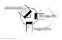


Sources:
- United States Patent and Trademark Office - verify current appl. status at the USPTO↗
Recent applications in this class:
- » 20250283734 2025-09-11
POSITION DETECTION DEVICE AND ACTUATOR - » 20250277678 2025-09-04
ROTARY SENSOR DEVICE, ROTARY SENSOR UNIT, AND INSTALLATION METHOD FOR ROTARY SENSOR DEVICE - » 20250271283 2025-08-28
LOCATING, IN A VEHICLE, ONE OR MORE PERIPHERALS - » 20250251257 2025-08-07
DYNAMIC RESOLUTION SENSOR - » 20250137816 2025-05-01
MAGNETIC YOKE ASSEMBLY AND SENSOR DEVICE - » 20250020486 2025-01-16
THREE AXIS MIRROR POSITION SENSING - » 20240426634 2024-12-26
NEAR-FIELD TRACKING - » 20240353239 2024-10-24
Method and system of one tactile sensor - » 20240288284 2024-08-29
PIEZOELECTRIC COIL WITH A SENSOR AND ELECTRONIC APPARATUS - » 20240288283 2024-08-29
MAGNETIC MARKER DETECTION METHOD AND DETECTION SYSTEM