OPTIMAL LOAD CURTAILMENT CALCULATING METHOD BASED ON LAGRANGE MULTIPLIER AND APPLICATION THEREOF

Description

CROSS-REFERENCE TO RELATED APPLICATION

This Application is a national stage application of PCT/CN2019/103669. This application claims priorities from PCT Application No. PCT/CN2019/103669, filed Aug. 30, 2019, and from the Chinese patent application 201910805095.7, filed Aug. 29, 2019, the contents of which are incorporated herein in the entirety by reference.

TECHNICAL FIELD

The present invention relates to the field of power system reliability assessment, and more particularly to an optimal load curtailment calculating method based on Lagrange multiplier and an application thereof in power system reliability assessment.

BACKGROUND OF THE PRESENT INVENTION

Energy security is a priority area of national security for all countries and an overarching and strategic issue concerning the national economy and people's livelihood. Power system is a main energy supply system, the primary objective of which is to supply users with safe, reliable and low-cost electricity. Owing to environmental impact, component aging, etc., power system components may fail randomly, which can cause power outages and load curtailment. This is a risk source of the power system. Both the probability and the impact of system failure should be considered in power system reliability assessment, and quantitatively assessing the power system risks with reliability indices is of great guiding significance for the planning, design, operation, and maintenance of power systems.

In recent years, with the rapid development of renewable energy such as wind energy and photovoltaic energy, the randomness and intermittence of the generation system are greatly enhanced. As a result, it brings more uncertainties in the power system reliability assessment. Moreover, the differences of load curves in different industries and regions increase with the development of society and division of labor. Thus, it is necessary to use various load curves to describe the actual time-varying loads of the power system, which increases the difficulties of reliability assessment. In general, traditional reliability assessment methods tend to use a unified probability distribution of load and renewable energy output, however, a great error often appears when load types and distributed energy resources become more various and complex. Therefore, different probability distributions should be used for different loads and renewable generations, to provide more accurate power system reliability assessment results.

However, multiple types of loads and renewable generations can lead to a myriad of system states. With the expansion of power systems, the exponentially growing system states will impose a large computational burden for the reliability assessment. Most existing researches like sorting and filtering, variance reduction, clustering, etc., focus on reducing the number of system states to be analyzed. To this end, only the representative states are selected and analyzed in order to improve the efficiency of reliability assessment. Nevertheless, owing to the system scale and limitation of accuracy, it inevitably entails a huge number of selected system states to analyze, which seriously restricts the efficiency of power system reliability assessment and cannot satisfy the requirements of efficiency and accuracy for online applications. Therefore, an efficient and accurate reliability assessment method for power systems with multiple types of loads and renewable generations is a technical problem needed to be solved in this field

SUMMARY OF THE PRESENT INVENTION

An objective of the present invention is to overcome the defects o the prior art, and to provide an optimal load curtailment calculating method based on Lagrange multiplier and an application thereof in power system reliability assessment. The method uses the Lagrange multiplier to calculate the optimal load curtailment and other impacts of system states to be assessed, which can speed up the system state analysis and thus improves the overall efficiency of power system reliability assessment.

The present invention solves the practical problems by adopting the following technical solutions.

An optimal load curtailment calculating method based on Lagrange multiplier includes the following steps:

Step 1: inputting all system states s to be analyzed for the reliability assessment, and establishing corresponding optimal load curtailment models, namely:

min c^T x

s.t. Ax=b,x≥0  (1)

Where x is a variable vector; A is a coefficient matrix; b is a right-hand-side vector; and c is a cost coefficient vector;

Step 2: classifying the above optimal load curtailment models into a plurality of sets by the Lagrange multiplier λ_s; and

Step 3: solving all the optimal load curtailment models in each set by the Lagrange multiplier λ_s of the set, to obtain optimal load curtailments f_{LC_s} of the system states.

Wherein, the step 2 includes following steps:

comparing an unclassified optimal load curtailment model with a classified one, and the two models belong to the same set if the Lagrange multipliers of the two models are the same;

determining whether the Lagrange multipliers of the two optimal load curtailment models are the same includes following steps:

adopting the judgment criterion to determine whether the different vectors A, b and c of the two models will lead to different Lagrange multipliers λ_s;

the maximum time of judgment is proposed, if it is exceeded, an optimal load curtailment model with the same Lagrange multiplier λ_s is not found, and this optimal load curtailment model is regarded as a single set; and

comparing and judging the values A, b and c of the two models in descending order according to the similarity thereof.

In Step 2, the Lagrange multipliers λ_s of all the optimal load curtailment models in each set are the same.

In the “comparing an unclassified optimal load curtailment model with a classified one” of Step 2, the Lagrange multiplier of the classified optimal load curtailment model is calculated by an optimization calculation method.

The Step 3 includes the following steps:

calculating the optimal load curtailments f_{LC_s} of the system states s by the Lagrange multipliers λ_s:

f_{LC_s}=λ_sb  (2)

Where b can be obtained from the optimal load curtailment model established in Step 1.

To solve the problems of the prior art, the following technical solution is also adopted in the present invention.

An application of the optimal load curtailment calculating method based on Lagrange multiplier in power system reliability assessment is provided. Specifically, the optimal load curtailment calculating method based on Lagrange multiplier is applied in power system reliability assessment to establish a power system reliability assessment device which includes an input and initialization module, a system state selection module, a state impact analysis module, and a reliability indices calculation module.

Module A. the input and initialization module is configured to input power system data, component reliability data and preset parameters of reliability assessment methods, including topological structure, branch parameters, component parameters, load data, renewable generation locations, renewable generation output data, and reliability parameters of components.

Module B. the system state selection module is configured to select the system states to be analyzed for the reliability assessment, including component contingency state, load time sequence state, and renewable generation output time sequence state. The system state selection method specifically includes State Enumeration (SE) technique, Monte Carlo Simulation (MCS) method, and improved methods of the SE technique and the MCS method.

Module C. the state impact analysis module is configured to analyze the impact of the system states selected by the Module B. The present invention computes the impact of the contingency state by the optimal load curtailment calculating method based on Lagrange multipliers and represents the impact by the load curtailments and all related indices.

Module D. the reliability indices calculation module is configured to compute the reliability indices of the power system based on the impact analysis results of the system states.

The advantages and beneficial effects of the present invention are as follows.

The core idea of the present invention, a Lagrange multiplier-based optimal load curtailment calculating method and application thereof in power system reliability assessment, is to establish Lagrange-multiplier-based linear functions between the optimal load curtailments and the system states. The iterative optimization processes of the traditional optimal load curtailment calculating method are substituted with the simple matrix multiplications. Thus, it can greatly reduce the amount of computation, improve the calculation speed without compromising the calculation accuracy. We can achieve an efficient and accurate reliability assessment for power systems with multiple types of loads and renewable generations. Moreover, the present invention has good compatibility. Since the idea of the present invention is to speed up the state analysis process of a single state, rather than to reduce the number of system states, the present invention can be integrated with a lot of existing research to obtain a more efficient and accurate reliability assessment method.

BRIEF DESCRIPTION OF THE DRAWINGS

The present invention includes the drawings illustrated herein, which are used to provide a further understanding of the embodiments thereof. The drawings of the present invention are not meant to limit the embodiments of the present invention.

FIG. 1 is a flowchart of an optimal load curtailment calculating method based on Lagrange multiplier;

FIG. 2 is an application flowchart of the optimal load curtailment calculating method based on Lagrange multiplier in power system reliability assessment;

FIG. 3 is a topological structure diagram of the RTS79 system;

FIG. 4(a) is an annual load curve of the first load (LA);

FIG. 4(b) is an annual load curve of the second load (LB);

FIG. 4(c) is an annual load curve of the third load (LC);

FIG. 5(a) is an annual output curve of photovoltaic power;

FIG. 5(b) is an annual output curve of wind power;

FIG. 6 is a comparison of relative errors of EENS indices by four methods for the RTS-79 system reliability assessment in Scenario 1;

FIG. 7 is a comparison of relative errors of EENS indices by four methods for the RTS-79 system reliability assessment in Scenario 2;

FIG. 8 is a topological structure diagram of the IEEE118-bus system;

FIG. 9 is a comparison of relative errors of EENS indices by four methods for the IEEE118-bus system reliability assessment in Scenario 1;

FIG. 10 is a comparison of relative errors of EENS indices by four methods for the IEEE118-bus system reliability assessment in Scenario 2; and

FIG. 11 is a block diagram illustrating an exemplary computing system in which the present system and method can operate.

DETAILED DESCRIPTION OF THE PRESENT INVENTION

In order to make the purposes, technical solutions and advantages of the present invention more clear, a further description of the optimal load curtailment calculating method based on Lagrange multiplier and an application thereof in power system reliability assessment is presented with reference to the embodiments thereof and accompanying drawings.

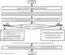
An optimal load curtailment calculating method based on Lagrange multiplier, as shown in FIG. 1, includes steps as follows.

Step 1: input the data related to system states s to be analyzed for the reliability assessment, specifically including the topological structure of power system, branch parameters, component parameters, load data of system states to be analyzed, renewable generations locations, renewable energy output levels, and failure components.

Step 2: optimal load curtailment models are established based on the system states s in the Step 1, and transformed into standard form by using the slack variables and surplus variables.

In each optimal load curtailment model, the minimum load curtailment is the objective function, active and reactive power output of generations, node voltage, and phase angle are used as variables, and node power balance, branch power flow limits, and upper and lower limits of variables are used as equality and inequality constraints. The model can be a DC model, a linearized AC model, and an AC model. These models are transformed into the standard model by introducing slack variables and surplus variables:

min c^Tx

s.t. Ax=b,x≥0  (1)

where x is the voltage, phase angle, power injection, slack variables, and surplus variables of the buses; A is a coefficient matrix, which represents the topological relation of the system and the slack relation of the variables; b is the branch power flow limits, the upper and lower limits of variables and the power balance value of the buses; and c is a cost coefficient vector such as penalty cost of load curtailments.

Step 3: the standard optimal load curtailment model in Step 2 is used to determine whether a system state s of the Step 1 belongs to a co-Lagrange-multiplier set (COLM-set). If so, the Lagrange multiplier λ_s of the system state s is obtained, go to Step 4B, otherwise, go to Step 4A.

If the system state from the Step 1 is the first system state to be analyzed, i.e., the optimal load curtailment calculating method based on Lagrange multiplier has not been performed before, Step 4A can be performed directly.

The Step 3 specifically includes the following steps: comparing the standard optimal load curtailment model in the Step 2 with the existing COLM-sets, and determining whether the system state s in the Step 1 belongs to a COLM-set. The model structure of the system state s is similar to that of the system state to be compared with, but there may be several differences in the values of the models. Thus, several judgment criteria are adopted depending on where the differences occur.

{circle around (1)} If the difference occurs in the cost coefficient vector c, it is assumed that the model in the Step 2 is c+Δc, and the model corresponding to the system state to be compared with is the vector c. If formula (2) is met, the two system states belong to the same COLM-set.

(c+Δc)^T−(c_BΔc_B)^TB⁻¹A≤0  (2)

As the cost coefficient vector c is different, the Lagrange multiplier λ_s of the system state s in the Step 1 is:

λ_s=(c_B+Δc_B)^TB⁻¹  (3)

{circle around (2)} If the difference occurs in the branch power flow limits b, it is assumed that the model in the Step 2 is b+Δb, and the model corresponding to the system state to be compared with is the branch power flow limits b. If formula (4) is met, the two system states belong to the same COLM-set.

B⁻¹(b+Δb)≥0  (4)

The Lagrange multiplier λ_s of the system state s in the Step 1 is:

λ_s=c^T_BB⁻¹  (5)

{circle around (3)} If the difference occurs in a column vector p_k in the coefficient matrix A, it is assumed that the model in the Step 2 is p_k+Δp_k, and the model corresponding to the system state to be compared with is the column vector p_k. If the column vector p_k does not belong to the optimal basis B, (i.e., the corresponding variable x_k is not the basic variable), and formula (6) is met, the two system states belong to the same COLM-set.

c_k−c_B^TB⁻¹(p_k+Δp_k)≤0  (6)

where c_k is the cost coefficient of the corresponding variable x_k. The Lagrange multiplier λ_s of the system state s in the Step 1 is:

λ_s=c_B^TB⁻¹  (7)

{circle around (4)} If the variable x changes, it is assumed that a new variable x_n+1 is added to the model of the system state to be compared in the Step 2. The cost coefficient c_n+1 and coefficient matrix column vector p_n+1 are added accordingly. If formula (8) is met, the two system states belong to the same COLM-set.

c_n+1−c_B^TB⁻¹p_n+1≤0  (8)

The Lagrange multiplier λ_s of the system state s in the Step 1) is:

λ_s=c_B^TB⁻¹  (9)

Based on the above judgment criteria, if the COLM-set to which the system state s in the Step 1 belongs, is found, go to Step 4B, otherwise, go to Step 4A.

Step 4A: the optimal load curtailment model established in the Step 2 is solved by the traditional optimal power flow algorithms, to obtain the optimal load curtailments f_{LC_s} of the system states s in the Step 1, and a new COLM-set is established based on this system state.

The specific method is as follows: the optimal load curtailment model (1) established by the system state s is solved by the traditional optimization calculating method, and the optimal load curtailment f_{LC_s} of the system state s is obtained. Meanwhile, the optimal solution x* can be divided into basic variable x_B and non-basic variable x_N, so the model (1) can be expressed as:

min ⁡ [ c B c N ] T ⁡ [ x B x N ] ⁢ ⁢ s . t . ⁢ [ B N ] ⁡ [ x B x N ] = b , x * ≥ 0 ( 10 )

where the optimal basis B and the non-optimal basis N correspond to the optimal basic variable X_B and the non-optimal basic variable x_N, respectively. Similarly, the cost coefficient vector c and the optimal solution x* in the model (1) are expressed as [c_B, c_N] and [x_B, x_N]^T, respectively.

Further, the equality constraint Ax=b can be expressed as:

Bx_B+Nx_N=b  (11)

where the non-basic variable x_N is zero and the optimal basis B is invertible, the solution of the model (1) can be expressed as:

min f_{LC_s}=c_B^TB⁻¹b

s.t. x_B=B⁻¹b, x*≥0  (12)

Where f_{LC_s} is an objective function value corresponding to the optimal solution x*, that is, the optimal load curtailment f_{LC_s} of the system state s.

The Lagrange multiplier λ_s in the model (1) of the system state s is:

λ_s=c_B^TB⁻¹  (13)

The optimal basis B, the optimal basic variable x_B, the cost coefficient c_B corresponding to the optimal basis, the coefficient matrix A, the Lagrange multiplier λ and the right-hand-side vector b, which are obtained from the solving process of the optimal load curtailment model, are stored to establish a COLM-set in which all the system states have the same Lagrange multiplier λ_s. This COLM-set will be used in the Step 3 of the optimal load curtailment calculating method based on Lagrange multiplier.

Step 4B: the optimal load curtailment f_{LC_s} of the system state s from the Step 1 is calculated based on the Lagrange multiplier λ_s determined in Step 3:

f_{LC_s}=λ_sb  (14)

where the vector b can be determined according to the optimal load curtailment model established in the Step 2.

An application of the optimal load curtailment calculating method based on Lagrange multiplier in power system reliability assessment is provided, as shown in FIG. 2. Specifically, the optimal load curtailment calculating method based on Lagrange multiplier is applied in power system reliability assessment to establish a power system reliability assessment device which includes an input and initialization module, a system state selection module, a state impact analysis module and a reliability indices calculation module.

Module A. the input and initialization module is configured to input power system data, component reliability data, and preset parameters of reliability assessment methods, including topological structure, branch parameters, component parameters, load data, renewable generations locations, renewable generations output data, reliability parameters of components.

Module B. the system state selection module is configured to select the system states to be analyzed for the reliability assessment, including component contingency state, load time sequence state, and renewable generation output time sequence state. The system state selection method specifically includes State Enumeration (SE) technique, Monte Carlo Simulation (MCS) method, and improved methods of the SE technique and the MCS method.

Module C. the state impact analysis module is configured to analyze the impact of the system states selected by Module B. The present invention computes the impact of the contingency state by the optimal load curtailment calculating method based on Lagrange multiplier, and represents the impact using the load curtailments and all related indices.

Module D. the reliability indices calculation module is configured to compute the reliability indices of the power system based on the impact analysis results of the states.

The reliability index R is calculated by the following formula:

R = ∑ s ∈ Ω ⁢ I ⁡ ( s ) ⁢ P ⁡ ( s ) ( 15 )

where I(s) is an impact function of the state s, such as load curtailment; and Ω is a set of system states.

In the SE technique and its related approaches, the probability P(s) of the system state s is:

P ⁡ ( s ) = ∏ i = 1 N f ⁢ u i ⁢ ∏ j = 1 N - N f ⁢ a j ( 16 )

where N_f is the number of failed components in the system state s.

In the MCS method and its related calculating methods, the sampling frequency P(s) of the system state s can be expressed as:

P ⁡ ( s ) = m ⁡ ( s ) M ( 17 )

where M is the total number of samples, and m(s) is the number of occurrences of system state s.

The reliability index is determined by the corresponding state impact function I(s), and the common reliability indices include: probability of load curtailments (PLC), expected energy not supplied, (EENS), average duration of load curtailments (ADLC), and Average Interruption Duration Index (ASAI), PLC and EENS are often used in practice as reliability indices which are obtained from formula (15):

EENS = T ⁢ ∑ s ∈ Ω ⁢ I L ⁢ C ⁡ ( s ) ⁢ P ⁡ ( s ) ( 18 ) PLC = ∑ s ∈ Ω ⁢ I L ⁢ C ⁢ F ⁡ ( s ) ⁢ P ⁡ ( s ) ( 19 )

where T is the assessment period; I_LC(s) is the load curtailments of the system state s; and I_LCF(s) is:

I L ⁢ C ⁢ F ⁡ ( s ) = { 1 , I L ⁢ C ⁡ ( s ) > 0 0 , I L ⁢ C ⁡ ( s ) = 0 ( 20 )

In the Impact-increment-based State Enumeration Technique (IISE), the reliability index R is calculated by the following formula:

R = ∑ k = 0 N ⁢ ∑ s ∈ Ω s k ⁢ Δ ⁢ ⁢ P s ⁢ Δ ⁢ I s ( 21 )

where N is the total order of reliability assessment; and k is the fault order of the system state s.

The impact increment ΔI_s of the system state s is:

Δ ⁢ I s = ∑ k = 0 n s ⁢ ( - 1 ) n s - k ⁢ ∑ v ∈ Ω s k ⁢ I v ( 22 )

where n_s is the number of failure components of the system state s; Ω_s is the total sets of contingency states within n_s-order of the system state s; and Ω_s^k is a k-order subset of Ω_s:

{ Ω s = { v  ⁢ v ⋐ s , Card ⁡ ( v ) ⁢ = 0 , 1 , 2 , … ⁢ , n s } Ω s k = { v ⁢ 1 ⁢ v ⋐ s , Card ( v ) ⁢ = k } Ω s k ⊆ Ω s   ( 23 )

where Card(v) represents the number of failure components in the state v. If k=0, Ω_s^k=ϕ.

The probability of impact increments ΔP_s of the system state s is:

Δ ⁢ P s = ∏ i ∈ Φ s ⁢ u i ( 24 )

where ϕ_s is a set of failure components in the system state s, and ΔP_s=0 if the system state s is a non-fault state.

For the embodiment of the present invention, the RTS79 system is used as an example, and its system topology diagram is shown in FIG. 3. The test system includes 24 buses, 33 generator units and 38 branches. The total generation capacity and the load are 34.05 MW and 28.5 MW, respectively. The computer hardware configuration of the embodiment includes Intel Xeon Platinum 8180 CPU (ES) 28×1.8 GHz and 128 GB RAM. The operating system is Windows 10, and the simulation software is MATLAB2018a.

Three test scenarios are considered to highlight the applicability of the present invention.

Scenario 1 (S1): a unified load curve, and conventional generators;

Scenario 2 (S2): three types of load curves, and conventional generators;

Scenario 3 (S3): three types of load curves, conventional generators, photovoltaics (PV) and wind turbines (WT);

The unified load curve is calculated proportionally by three annual load curves (LA, LB, LC) according to the load proportion. The three annual load curves are the actual load curves of the northeast region, Edmonton region, and southern region of Alberta, Canada, as shown in FIGS. 4(a)-4(b). The annual output curves of PV and WT are obtained from National Wind Technology Center(NREL), as shown in FIGS. 5(a)-5(b). The node load types and renewable energy node settings in scenarios 2 and 3 are shown in Table 1.

TABLE 1
Node Settings of Scenarios 2 and 3
(RTS79)

	Type	Node
	LA	1, 2, 4, 5, 6, 7, 8
	LB	15, 16, 18, 19, 20
	LC	3, 9, 10, 13, 14
	PV	13
	WT	7

In the embodiment of the present invention, an optimal load curtailment calculating method based on Lagrange multiplier is applied in the reliability assessment to evaluate the reliability level of composite generation and transmission systems. The reliability index is EENS and the DC model is adopted as the optimal load curtailment model. Combined with the impact increment technique and clustering method, the proposed method is compared with the traditional SE technique and MCS method to verify the efficiency, accuracy and compatibility.

The input system includes node types, active loads, reference voltage, and upper and lower limits of the voltage of the RTS79 system; location, upper and lower limits of the active power output of generators; node topological relation, reactance, and power flow limits of the branches, as shown in Table 5. The three annual load curves and annual output curves of PV and WT are shown in FIGS. 4(a)-4(c) and 5(a)-5(b).

According to the above steps of the present invention, different methods are adopted to assess the reliability of power systems in the three scenarios. For the MCS method, the sampled system state number is 5×10⁷, and the results of MCS are treated as a benchmark to evaluate other methods. The results are shown in Table 2.

TABLE 2
Reliability Assessment Results of Four Methods (RTS79)

				EENS	Average
		Number of	EENS	Relative	Number of	CPUTime
Scenario	Method	Clusters	(MWh/y)	Error (%)	COLM-sets	(s)

S1	MCS	8760	4105.29	0	—	3451
	LM-IISE	8760	4155.16	1.21	1.77	83
	LMSE		2203.35	46.33	—	83
	SE		2203.35	46.33	—	21746
	LM-IISE	100	4153.84	1.18	1.66	9
	LMSE		2202.61	46.35	—	9
	SE		2202.62	46.35	—	237
	LM-IISE	10	3989.10	2.83	1.39	7
	LMSE		2125.43	48.2270	—	7
	SE		2125.43	48.2270	—	25
S2	MCS	8760	4131.43	0	—	3366
	LM-IISE	8760	4250.96	2.89	1.49	143
	LMSE		2259.71	45.30	—	143
	SE		2259.71	45.30	—	21908
	LM-IISE	100	4144.41	0.31	1.32	8
	LMSE		2205.55	46.62	—	8
	SE		2205.55	46.62	—	236
	LM-IISE	10	3787.41	8.33	1.15	7
	LMSE		2000.11	51.59	—	7
	SE		2000.11	51.59	—	25
S3	MCS	8760	3566.93	0	—	3851
	LM-IISE	8760	3599.31	0.91	2.25	209
	LMSE		1894.53	46.89	—	209
	SE		1894.53	46.89	—	21869
	LM-IISE	500	3437.33	3.63	1.97	12
	LMSE		1802.63	49.46	—	12
	SE		1802.62	49.46	—	1216
	LM-IISE	100	3190.06	10.57	1.78	21
	LMSE		1659.17	53.4846	—	21
	SE		1659.17	53.4846	—	241

Table 2 shows the reliability assessment results by EENS. It can be seen that the optimal load curtailment based on Lagrange multiplier has an outstanding advantage in the calculation speed which is more than 10 times faster than that of the traditional SE technique. It can be seen from the average number of COLM-sets that the step 4B is performed about twice in the entire solving process (i.e., the optimal power flow problem is solved only twice), and other states are solved by Lagrange multiplier. As a result, the present invention saves a lot of calculation time. Owing to the compatibility of the present invention, the optimal load curtailment calculating method based on Lagrange multiplier can be combined with the IISE method (LM-IISE). In terms of calculation accuracy, the relative error of LM-IISE is less than 3%, which is close to the accuracy of the MCS method, so that the proposed method can satisfy the requirements of practical application. In conclusion, combined with the IISE technique and the clustering algorithm, the present invention can achieve an error less than 4% within 10 seconds, which is far superior to the other three methods in terms of both speed and accuracy.

FIGS. 6 and 7 show the comparisons of the relative errors of reliability indices by the four methods for the RTS-79 system in the scenarios 1 and 2, respectively. In the figures, the closer to the lower-left corner the position of the method is, the more effective the method is. As shown in FIGS. 6 and 7, the computation speed of the method can be increased by more than 10 times, and the calculation accuracy remains unchanged. By integrating with the IISE technique and the clustering method, the position of LM-IISE (100) is located at the lower left of others. It can be seen from the relative error convergence curve that the MCS method spends more than 100 seconds when its relative error drops to 1%, while such precision can be reached by the method within 10 seconds.

Therefore, the optimal load curtailment method based on Lagrange multiplier according to the present invention has an outstanding advantage in the calculation speed, and the application thereof in traditional reliability assessment methods can achieve higher accuracy and efficiency than those of the traditional reliability assessment methods.

The implementation process and practical effects of the present invention are illustrated by another embodiment. The IEEE 118-bus system is tested in this embodiment, and its system topology diagram is shown in FIG. 8. The test system includes 118 buses, 54 generator units, 186 branches, 54 generation buses, and 64 load buses. The total generation capacity and the load are 9,966MW and 4,242 MW, respectively. The node load types and renewable energy node settings in the scenarios 2 and 3 are shown in Table 3. The system configuration and test scenario settings are the same as those of the previous embodiment.

In the embodiment of the present invention, an optimal load curtailment calculating method based on Lagrange multiplier is applied in reliability assessment to evaluate the reliability level of composite generation and transmission system. The reliability index is EENS, and the DC model is adopted as the optimal load curtailment model. Combined with the impact increment technique and clustering method, the proposed method is compared with the traditional SE technique and MCS method to verify the efficiency, accuracy, compatibility, and practicability in large-scale systems.

The input system includes node types, active loads, reference voltage, and upper and lower limits of voltage of the IEEE 118-bus system; location, upper and lower limits of the active output of generators; node topological relation, reactance, and power flow limits of the branches, as shown in Table 6. The three annual load curves and annual output curves of PV and WT are shown in FIGS. 4(a)-4(c) and 5(a)-5(b).

TABLE 3
Node Settings of Scenarios 2 and 3 (IEEE118-bus)

Type	Node
LA	82, 83, 84, 85, 86, 87, 88, 89, 90, 91, 92, 93, 94, 95, 96, 100,
	101, 102, 103, 104, 105, 106, 107, 108, 109, 110, 111, 112
LB	1, 2, 3, 4, 5, 6, 7, 8, 9, 10, 11, 12, 13, 14, 15, 16, 17, 18, 19,
	20, 21, 22, 23, 24, 25, 26, 27, 28, 29, 30, 31, 32, 70, 71, 72,
	73, 74, 75, 113, 114, 115, 117
LC	33, 34, 35, 36, 37, 38, 39, 40, 41, 42, 43, 44, 45, 46, 47, 48,
	49, 50, 51, 52, 53, 54, 55, 56, 57, 58, 59, 60, 61, 62, 63, 64,
	65, 66, 67, 68, 69, 76, 77, 78, 79, 80, 81, 97, 98, 99, 116, 118
PV	1, 12, 25, 34, 49, 61, 70, 77, 90, 103, 111
power
Wind	6, 18, 27, 40, 55, 65, 73, 85, 92, 105, 113
power

According to the above steps of the present invention, different methods are adopted to assess the reliability of power systems in the three scenarios. For the MCS method, the sampled system state number is 10⁸, and the results of MCS are treated as a benchmark to evaluate other methods. The results are shown in Table 4.

Table 4 shows the reliability assessment results by EENS. It can be seen that the optimal load curtailment based on Lagrange multiplier has an outstanding advantage in the calculation speed. When the number of clusters is greater than 100, the calculation speed of the present invention is more than 10 times faster than that of the traditional SE technique. It can be seen from the average number of COLM-sets that the step 4B is performed about five times in the entire solving process, (i.e., the optimal power flow problems are solved only five times), and other states are solved by Lagrange multiplier. As a result, it can save a lot of calculation time. Owing to the compatibility of the present invention, the optimal load curtailment calculating method based on Lagrange multiplier can be combined with the IISE method (LM-IISE). In terms of calculation accuracy, the relative error of LM-IISE is less than 5%, which is close to the accuracy of the MCS method, so that the proposed method can satisfy the requirements of practical application. In conclusion, combined with the IISE technique and the clustering algorithm, the present invention can achieve an error of about 5% within 100 seconds, which is far superior to the other three methods in terms of both speed and accuracy.

TABLE 4
Reliability Assessment Results of Four Methods (IEEE118-bus)

				EENS	Average
		Number of	EENS	Relative	Number of	CPU
Scenario	Method	clusters	(MWh/y)	Error (%)	COLM-sets	time (s)

S1	MCS	—	257.39	0	—	24831
	LM-IISE	8760	249.93	2.90	2.55	399
	LMSE		170.86	33.62	—	399
	SE		170.86	33.62	—	65031
	LM-IISE	100	249.92	2.90	2.43	62
	LMSE		170.86	33.62	—	62
	SE		170.86	33.62	—	747
	LM-IISE	10	243.81	5.27	2.15	50
	LMSE		166.14	35.45	—	50
	SE		166.14	35.45	—	77
S2	MCS	—	243.04	0	—	24802
	LM-IISE	8760	237.91	2.11	4.97	588
	LMSE		165.12	32.06	—	588
	SE		165.12	32.06	—	64910
	LM-IISE		233.02	4.12	3.98	98
	LMSE	100	161.66	33.48	—	98
	SE		161.67	33.48	—	604
	LM-IISE		209.67	13.73	2.82	67
	LMSE	10	145.47	40.15	—	67
	SE		145.47	40.15	—	63
S3	MCS	—	240.06	0	—	26946
	LM-IISE		234.05	2.50	4.20	768
	LMSE	8760	162.95	32.12	—	768
	SE		162.95	32.12	—	65219
	LM-IISE		225.94	5.88	3.38	113
	LMSE	500	157.24	34.50	—	113
	SE		157.24	34.50	—	3694
	LM-IISE		214.11	10.81	2.73	73
	LMSE	100	149.36	37.78	—	73
	SE		149.36	37.78	—	734

FIGS. 9 and 10 show the comparison of the relative errors reliability indices by the four methods for the IEEE118-bus system in the scenarios 1 and 2, respectively. In the figures, the closer to the lower-left corner the position of the method is, the more effective the method is. As shown in the FIGS. 9 and 10, the computation speed of the method can be increased by more than 10 times, and the calculation accuracy remains unchanged. By integrating with the IISE technique and the clustering method, the position of LM-IISE (100) is located at the lower left of others. It can be seen from the relative error convergence curve that the present invention is slightly superior to the MCS method. This is because that the SE technique is not suitable for large-scale system reliability assessment. We would achieve a better performance if the present invention is applied in the MCS method.

Therefore, the optimal load curtailment method based on Lagrange multiplier has an outstanding advantage in the calculation speed, and the application thereof in traditional reliability assessment methods can achieve higher accuracy and efficiency than those of the traditional reliability assessment methods.

Referring to FIG. 11, the methods and systems of the present disclosure can be implemented on power system reliability assessment device 1100, including one or more computers. The methods and systems disclosed can utilize one or more computers to perform one or more functions in one or more locations. The processing of the disclosed methods and systems can also be performed by software components stored on, for example, without limitation, mass storage device 1115. The disclosed systems and methods can be described in the general context of computer-executable instructions such as program modules including one or more of, Input and Initialization Module 1125, System State Selection Module 1130, State Impact Analysis Module 1135, Reliability Indices Calculation Module 1140, etc. being executed on processor 1110 of power system reliability assessment device 1100. Input and Initialization Module 1125 is configured to input power system data 1165, component reliability data 1170, and preset parameters 1175 of reliability assessment methods, including topological structure, branch parameters, component parameters, load data, renewable generation locations, renewable generation output data, and reliability parameters of components. System State Selection Module 1130 is configured to select the system states to be analyzed for the reliability assessment, including component contingency state, load time sequence state, and renewable generation output time sequence state. State Impact Analysis Module 1135 is configured to analyze the impact of the system states selected by the module B using the optimal load curtailment calculating method of Lagrange multiplier according to claim 1, and represents the impact by the load curtailments and all related indices. Reliability Indices Calculation Module 1140 is configured to compute the reliability indices of the power system based on the impact analysis results of the system states. These program modules can be stored on mass storage device 1115 of power system reliability assessment device 1100 co-located with power system 1185 or remotely located respect to power system 1185. Each of the operating modules can comprise elements of the programming and the data management software.

Program code for an optimal load curtailment calculating method based on a Lagrange multiplier may be stored on one or more of mass storage device 1115 and system memory 1160 that, when executed by processor 1110 cause processor 1110 to carry out steps 1-3, as described with reference to FIG. 1 above.

The components of power system reliability assessment device 1100 include, but are not limited to, one or more processors or processing units 1110, system memory 1160, mass storage device 1115, operating system 1120, system memory 1160, display adapter 1145, Input/Output Interface 1150, network adaptor 1155, and system bus 1190 that couples various system components. Power system reliability assessment device 1100 and power system 1185 may communicate via wired or wireless network 1180 at physically separate locations as a fully distributed system, or power system reliability assessment device 1100 may be integrated into power system 1185. By way of example, power system reliability assessment device 1100 may be a personal computer, a portable computer, a smart device, a network computer, a peer device, or other common network node, and so on. Logical connections between one or more computers and one or more power systems can be made via network 1180, such as a local area network (LAN) and/or a general wide area network (WAN).

It should be understood by those of skills in the art that the drawings and tables are merely schematic diagrams of a preferred embodiment, and the order of the above embodiments in the present invention is only for description, and not meant to the superiority and inferiority of the embodiments.

The proposes, technical solutions and beneficial effects of the present invention are further described in detail by the embodiments mentioned above. It should be understood that those described above are merely preferred embodiments of the present invention, and are not intended to limit the protection scope of the present invention. Any modifications, equivalent substitutions and improvements made within the spirit and principle of the present invention shall fall into the protection scope of the present invention.

TABLE 5A
Bus Data of RTS79 System

		Active
	Bus	load
	Number	(MW)

	1	108
	2	97
	3	180
	4	74
	5	71
	6	136
	7	125
	8	171
	9	175
	10	195
	11	0
	12	0
	13	265
	14	194
	15	317
	16	100
	17	0
	18	333
	19	181
	20	128
	21	0
	22	0
	23	0
	24	0

TABLE 5B
Generator Data of RTS79 System

	Maximum
	Active
	Power
Bus	Output	Unavailability
Number	(MW)	(%)

1	20	10
1	20	10
1	76	2
1	76	2
2	20	10
2	20	10
2	76	2
2	76	2
7	100	4
7	100	4
7	100	4
13	197	5
13	197	5
13	197	5
14	0	0
15	12	2
15	12	2
15	12	2
15	12	2
15	12	2
15	155	4
16	155	4
18	400	12
21	400	12
22	50	1
22	50	1
22	50	1
22	50	1
22	50	1
22	50	1
23	155	4
23	155	4
23	350	8

TABLE 5C
Branch Data of RTS79 System

“From”	“To”		Transformer	Transmission
Bus	Bus	Reactance	Ratio	Limit	Unavailability
Number	Number	(p.u.)	(p.u.)	(MW)	(%)

1	2	0.0139		175	0.04382
1	3	0.2112		175	0.05819
1	5	0.0845		175	0.03766
2	4	0.1267		175	0.04450
2	6	0.1920		175	0.05476
3	9	0.1190		175	0.04336
3	24	0.0839	1.03	400	0.17504
4	9	0.1037		175	0.04108
5	10	0.0883		175	0.03880
6	10	0.0605		175	0.13168
7	8	0.0614		175	0.03423
8	9	0.1651		175	0.05020
8	10	0.1651		175	0.05020
9	11	0.0839	1.03	400	0.17504
9	12	0.0839	1.03	400	0.17504
10	11	0.0839	1.02	400	0.17504
10	12	0.0839	1.02	400	0.17504
11	13	0.0476		500	0.05020
11	14	0.0418		500	0.04895
12	13	0.0476		500	0.05020
12	23	0.0966		500	0.06525
13	23	0.0865		500	0.06149
14	16	0.0389		500	0.04769
15	16	0.0173		500	0.04142
15	21	0.0490		500	0.05146
15	21	0.0490		500	0.05146
15	24	0.0519		500	0.05146
16	17	0.0259		500	0.04393
16	19	0.0231		500	0.04268
17	18	0.0144		500	0.04017
17	22	0.1053		500	0.06776
18	21	0.0259	0.96	500	0.04393
18	21	0.0259		500	0.04393
19	20	0.0396		500	0.04769
19	20	0.0396		500	0.04769
20	23	0.0216	0.96	500	0.04268
20	23	0.0216		500	0.04268
21	22	0.0678		500	0.05647

TABLE 6A
Bus Data of IEEE 118-bus System

		Active
	Bus	load
	Number	(MW)

	1	51
	2	20
	3	39
	4	39
	5	0
	6	52
	7	19
	8	28
	9	0
	10	0
	11	70
	12	47
	13	34
	14	14
	15	90
	16	25
	17	11
	18	60
	19	45
	20	18
	21	14
	22	10
	23	7
	24	13
	25	0
	26	0
	27	71
	28	17
	29	24
	30	0
	31	43
	32	59
	33	23
	34	59
	35	33
	36	31
	37	0
	38	0
	39	27
	40	66
	41	37
	42	96
	43	18
	44	16
	45	53
	46	28
	47	34
	48	20
	49	87
	50	17
	51	17
	52	18
	53	23
	54	113
	55	63
	56	84
	57	12
	58	12
	59	277
	60	78
	61	0
	62	77
	63	0
	64	0
	65	0
	66	39
	67	28
	68	0
	69	0
	70	66
	71	0
	72	12
	73	6
	74	68
	75	47
	76	68
	77	61
	78	71
	79	39
	80	130
	81	0
	82	54
	83	20
	84	11
	85	24
	86	21
	87	0
	88	48
	89	0
	90	163
	91	10
	92	65
	93	12
	94	30
	95	42
	96	38
	97	15
	98	34
	99	42
	100	37
	101	22
	102	5
	103	23
	104	38
	105	31
	106	43
	107	50
	108	2
	109	8
	110	39
	111	0
	112	68
	113	6
	114	8
	115	22
	116	184
	117	20
	118	33

TABLE 6B
Generator Data of IEEE 118-bus System

	Maximum
	Active
	Power
Bus	output	Unavailability
Number	(MW)	(%)

1	100	0.015
4	100	0.015
6	100	0.015
8	100	0.015
10	550	0.015
12	185	0.015
15	100	0.015
18	100	0.015
19	100	0.015
24	100	0.015
25	320	0.015
26	414	0.015
27	100	0.015
31	107	0.015
32	100	0.015
34	100	0.015
36	100	0.015
40	100	0.015
42	100	0.015
46	119	0.015
49	304	0.015
54	148	0.015
55	100	0.015
56	100	0.015
59	255	0.015
61	260	0.015
62	100	0.015
65	491	0.015
66	492	0.015
69	805.2	0.015
70	100	0.015
72	100	0.015
73	100	0.015
74	100	0.015
76	100	0.015
77	100	0.015
80	577	0.015
85	100	0.015
87	104	0.015
89	707	0.015
90	100	0.015
91	100	0.015
92	100	0.015
99	100	0.015
100	352	0.015
103	140	0.015
104	100	0.015
105	100	0.015
107	100	0.015
110	100	0.015
111	136	0.015
112	100	0.015
113	100	0.015
116	100	0.015

TABLE 6C
Branch Data of IEEE 118-bus System

“From”	“To”		Transformer	Transmission	Unavail-
Bus	Bus	Reactance	ratio	limit	ability
Number	Number	(p.u.)	(p.u.)	(MW)	(%)

1	2	0.0999		175	0.04153
1	3	0.0424		175	0.03353
4	5	0.00798		500	0.02874
3	5	0.108		175	0.04265
5	6	0.054		175	0.03514
6	7	0.0208		175	0.03052
8	9	0.0305		500	0.03187
8	5	0.0267	0.9850	500	0.18
9	10	0.0322		500	0.03211
4	11	0.0688		175	0.0372
5	11	0.0682		175	0.03712
11	12	0.0196		175	0.03036
2	12	0.0616		175	0.0362
3	12	0.16		175	0.04989
7	12	0.034		175	0.03236
11	13	0.0731		175	0.0378
12	14	0.0707		175	0.03746
13	15	0.2444		175	0.06163
14	15	0.195		175	0.05475
12	16	0.0834		175	0.03923
15	17	0.0437		500	0.03371
16	17	0.1801		175	0.05268
17	18	0.0505		175	0.03465
18	19	0.0493		175	0.03449
19	20	0.117		175	0.0439
15	19	0.0394		175	0.03311
20	21	0.0849		175	0.03944
21	22	0.097		175	0.04112
22	23	0.159		175	0.04975
23	24	0.0492		175	0.03447
23	25	0.08		500	0.03876
26	25	0.0382	0.96	500	0.18
25	27	0.163		500	0.0503
27	28	0.0855		175	0.03952
28	29	0.0943		175	0.04075
30	17	0.0388	0.96	500	0.18
8	30	0.0504		175	0.03464
26	30	0.086		500	0.03959
17	31	0.1563		175	0.04937
29	31	0.0331		175	0.03223
23	32	0.1153		140	0.04367
31	32	0.0985		175	0.04133
27	32	0.0755		175	0.03813
15	33	0.1244		175	0.04493
19	34	0.247		175	0.06199
35	36	0.0102		175	0.02905
35	37	0.0497		175	0.03454
33	37	0.142		175	0.04738
34	36	0.0268		175	0.03136
34	37	0.0094		500	0.02894
38	37	0.0375	0.935	500	0.18
37	39	0.106		175	0.04237
37	40	0.168		175	0.051
30	38	0.054		175	0.03514
39	40	0.0605		175	0.03605
40	41	0.0487		175	0.0344
40	42	0.183		175	0.05309
41	42	0.135		175	0.04641
43	44	0.2454		175	0.06177
34	43	0.1681		175	0.05101
44	45	0.0901		175	0.04016
45	46	0.1356		175	0.04649
46	47	0.127		175	0.0453
46	48	0.189		175	0.05392
47	49	0.0625		175	0.03632
42	49	0.323		175	0.07256
42	49	0.323		175	0.07256
45	49	0.186		175	0.0535
48	49	0.0505		175	0.03465
49	50	0.0752		175	0.03809
49	51	0.137		175	0.04669
51	52	0.0588		175	0.03581
52	53	0.1635		175	0.05037
53	54	0.122		175	0.0446
49	54	0.289		175	0.06783
49	54	0.291		175	0.06811
54	55	0.0707		175	0.03746
54	56	0.00955		175	0.02896
55	56	0.0151		175	0.02973
56	57	0.0966		175	0.04107
50	57	0.134		10	0.04627
56	58	0.0966		175	0.04107
51	58	0.0719		175	0.03763
54	59	0.2293		175	0.05953
56	59	0.251		175	0.06254
56	59	0.239		175	0.06087
55	59	0.2158		175	0.05765
59	60	0.145		100	0.0478
59	61	0.15		175	0.0485
60	61	0.0135		50	0.02951
60	62	0.0561		50	0.03543
61	62	0.0376		175	0.03286
63	59	0.0386	0.96	500	0.18
63	64	0.02		500	0.03041
64	61	0.0268	0.985	500	0.18
38	65	0.0986		500	0.04135
64	65	0.0302		500	0.03183
49	66	0.0919		500	0.04041
49	66	0.0919		500	0.04041
62	66	0.218		175	0.05795
62	67	0.117		175	0.0439
65	66	0.037	0.935	500	0.18
66	67	0.1015		175	0.04175
65	68	0.016		500	0.02986
47	69	0.2778		175	0.06627
49	69	0.324		175	0.0727
68	69	0.037	0.935	500	0.18
69	70	0.127		500	0.0453
24	70	0.4115		175	0.08487
70	71	0.0355		175	0.03257
24	72	0.196		175	0.05489
71	72	0.18		175	0.05267
71	73	0.0454		175	0.03395
70	74	0.1323		175	0.04603
70	75	0.141		175	0.04724
69	75	0.122		500	0.0446
74	75	0.0406		175	0.03328
76	77	0.148		175	0.04822
69	77	0.101		175	0.04168
75	77	0.1999		175	0.05544
77	78	0.0124		175	0.02935
78	79	0.0244		175	0.03102
77	80	0.0485		500	0.03438
77	80	0.105		500	0.04224
79	80	0.0704		175	0.03742
68	81	0.0202		500	0.03044
81	80	0.037	0.935	500	0.18
77	82	0.0853		200	0.0395
82	83	0.03665		200	0.03273
83	84	0.132		175	0.04599
83	85	0.148		175	0.04822
84	85	0.0641		175	0.03655
85	86	0.123		500	0.04474
86	87	0.2074		500	0.05648
85	88	0.102		500	0.04182
85	89	0.173		175	0.05169
88	89	0.0712		500	0.03753
89	90	0.188		500	0.05378
89	90	0.0997		175	0.0415
90	91	0.0836		175	0.03926
89	92	0.0505		175	0.03465
89	92	0.1581		175	0.04962
91	92	0.1272		175	0.04532
92	93	0.0848		175	0.03943
92	94	0.158		175	0.04961
93	94	0.0732		175	0.03781
94	95	0.0434		175	0.03367
80	96	0.182		175	0.05295
82	96	0.053		175	0.035
94	96	0.0869		175	0.03972
80	97	0.0934		175	0.04062
80	98	0.108		175	0.04265
80	99	0.206		200	0.05628
92	100	0.295		175	0.06866
94	100	0.058		175	0.0357
95	96	0.0547		175	0.03524
96	97	0.0885		175	0.03994
98	100	0.179		175	0.05253
99	100	0.0813		175	0.03894
100	101	0.1262		175	0.04518
92	102	0.0559		175	0.03541
101	102	0.112		175	0.04321
100	103	0.0525		500	0.03493
100	104	0.204		175	0.05601
103	104	0.1584		175	0.04966
103	105	0.1625		175	0.05023
100	106	0.229		175	0.05948
104	105	0.0378		175	0.03289
105	106	0.0547		175	0.03524
105	107	0.183		175	0.05309
105	108	0.0703		175	0.03741
106	107	0.183		175	0.05309
108	109	0.0288		175	0.03164
103	110	0.1813		175	0.05285
109	110	0.0762		175	0.03823
110	111	0.0755		175	0.03813
110	112	0.064		175	0.03653
17	113	0.0301		175	0.03182
32	113	0.203		500	0.05587
32	114	0.0612		175	0.03614
27	115	0.0741		175	0.03794
114	115	0.0104		175	0.02908
68	116	0.00405		500	0.02819
12	117	0.14		175	0.0471
75	118	0.0481		175	0.03432
76	118	0.0544		175	0.0352