Data-Driven Liquid Loading Detection and Prediction

Description

CROSS-REFERENCE TO RELATED APPLICATIONS

This application claims priority to U.S. Provisional Application No. 63/631,588 filed Apr. 9, 2024 entitled “Data-Driven Liquid Loading Detection and Prediction”, which is incorporated herein by reference as if reproduced in its entirety.

TECHNICAL FIELD

The present disclosure relates to determining estimations of reservoir or well performance characteristics and, more particularly, to systems and methods for determining liquid loading.

BACKGROUND

Liquid loading in gas wells refers to the phenomenon where the production of natural gas is hindered by the accumulation of a liquid column (i.e., of condensate and/or water) in the wellbore. It results from the inability of gas to entrain the liquids to the surface. When the gas velocity is insufficient to carry the liquids to the surface then the liquid starts falling back into the wellbore creating additional backpressure due to the accumulated liquid column. This leads to the reduction of fluid inflow rate from the reservoir into the well caused by lower drawdown pressure. As the liquid accumulation increases further, the drawdown pressure becomes negligible and the well stops producing. Liquid loading is a persistent challenge encountered in onshore and offshore gas wells, particularly at low gas rates, where the accumulation of wellbore liquids leads to flow instabilities, operational disruptions, prolonged shut-ins leading to early well abandonment and reduced overall recovery. Typical liquid loading mitigation strategies such as velocity strings, well cycling, intermittent or permanent artificial lift, surfactants/soaps etc. involve additional cost and therefore, their operational success relies on selecting the right wells with proper understanding of expected critical rates at the right time.

There are correlation models that can be used to model this liquid loading phenomenon. However, the empirical correlations commonly used to detect liquid loading often lack precision in field applications due to oversimplified assumptions regarding liquid behavior and flow regime consistency. A need exists for a method for detecting and predicting liquid loading in a given well, which can be applied in a practical and automated manner.

BRIEF DESCRIPTION OF THE DRAWINGS

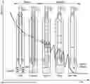
FIG. 1 is a schematic of example flow regimes.

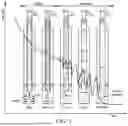
FIGS. 2A-2B are schematics of example models for liquid transportation.

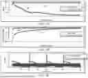
FIGS. 3A-3C are a set of plots representing comparisons between a liquid loaded well and a stable well.

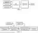
FIG. 4 is a schematic of an example workflow to determine critical gas rate.

FIG. 5 is a schematic of an example workflow to determine a time for liquid loading.

FIG. 6 is a plot representing a critical operating point for a well.

FIG. 7 is a plot representing an estimation of gas production before liquid loading.

FIGS. 8A-8D are a set of plots representing multiphase transient flow and an effect of liquid loading.

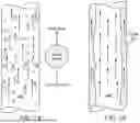
FIGS. 9A-9E are a set of plots representing liquid volume fraction at various stages of liquid loading.

FIGS. 10A-10B are a set of plots representing gas rates and wellhead pressures for stable flow.

FIG. 11 is a plot representing a comparison between empirical critical rates and calibration of the best critical rate for stable flow.

FIGS. 12A-12B are a set of plots representing gas rates and wellhead pressures.

FIG. 13 is a plot representing a comparison between empirical critical rates and calibration of the best critical rate for a liquid loaded well.

FIG. 14 is a plot representing changes in gas lift operations.

FIGS. 15A-15B are a set of plots representing gas rates and wellhead pressures.

FIG. 16 is a plot representing a comparison between critical gas rates, actual gas rates, and a corrected critical rate.

FIGS. 17A-17C are a set of plots representing comparisons between a liquid loaded well and a stable well.

FIGS. 18A-18B are a set of plots representing nodal analysis and material balance with forecasted parameters for predicting liquid loading.

FIG. 19 is a block diagram showing an example control unit in accordance with certain embodiments of the present disclosure.

While embodiments of this disclosure have been depicted and described and are defined by reference to exemplary embodiments of the disclosure, such references do not imply a limitation on the disclosure, and no such limitation is to be inferred. The subject matter disclosed is capable of considerable modification, alteration, and equivalents in form and function, as will occur to those skilled in the pertinent art and having the benefit of this disclosure. The depicted and described embodiments of this disclosure are examples only, and not exhaustive of the scope of the disclosure.

DETAILED DESCRIPTION

Illustrative embodiments of the present disclosure are described in detail herein. In the interest of clarity, not all features of an actual implementation may be described in this specification. It will of course be appreciated that in the development of any such actual embodiment, numerous implementation-specific decisions may be made to achieve the specific implementation goals, which may vary from one implementation to another. Moreover, it will be appreciated that such a development effort might be complex and time-consuming, but would nevertheless be a routine undertaking for those of ordinary skill in the art having the benefit of the present disclosure.

To facilitate a better understanding of the present disclosure, the following examples of certain embodiments are given. In no way should the following examples be read to limit, or define, the scope of the disclosure. Embodiments described below with respect to one implementation are not intended to be limiting.

The present disclosure relates to systems and methods for determining an onset of liquid loading and/or predicting a future onset time for liquid loading. The systems and methods may provide a data-driven approach for liquid loading detection and prediction (LLDP) that harnesses high-frequency gas rate and tubing head pressure measurements to identify the onset of liquid loading and use it to correct critical rates computed by empirical methods. The LLDP methodology may include the computation of diagnostic statistical proxy features, enabling the characterization of flow instability arising from liquid loading. Upon detection, subsequent adjustment to gas rates via feedback control may facilitate the determination of corrected critical rate by calibration of empirical correlations. This allows for prediction of when the reservoir energy will no longer be sufficient to lift the liquids combined with the corrected critical gas curve and estimate time to liquid loading.

The LLDP may provide a rapid and systematic approach for the detection, quantification, and prediction of liquid loading, utilizing readily available field data without relying on assumptions. By accurately identifying critical gas rates and optimizing artificial lift configurations, the LLDP method may offer a practical solution to the challenges posed by liquid loading in gas wells, thereby enhancing operational efficiency and maximizing production.

In one or more embodiments, liquid loading mitigation strategies may include: (1) installation of velocity strings (also referred to as “microstrings”) with smaller diameters to reduce the diameter of tubing to increase velocity; (2) well cycling to shut-in the well intentionally for a small duration of time to build near-wellbore pressure and later re-opening the well to lift the liquids out; (3) intermittent and/or permanent artificial lift with plungers, gas-assisted plungers, gas lift etc. by providing external energy to lift the liquids; (4) adding surfactants (i.e., soaps) to lighten the fluid density by forming a foam; (5) re-stimulating the well to reduce near-wellbore skin and/or increase well productivity; (6) re-completing or re-perforating the well to increase well productivity and produced gas velocity; or (7) reducing the wellhead pressure with a compressor to increase fluid velocity in the wellbore. However, successful design and operation of one or more of these strategies may rely on selecting the correct wells with proper understanding of expected critical rates at the right time.

Critical rate may be defined herein as the minimum gas rate required in the wellbore to lift the liquids. Due to buoyancy effects (i.e., the density difference between gas and liquid), it may be expected that the gas will flow faster than the liquid during vertical upward flow. Consequently, depending on each of their velocities, the gas and liquid will present different topological distributions or flow patterns inside the conduit. To understand liquid loading within the framework of multiphase flow, a user or operator may be required to know the typical flow regimes observed in vertical gas wells during gas-liquid flow, as shown in FIG. 1.

FIG. 1 shows an illustration of example flow regimes. At high gas flow rates with very low liquid-gas ratio, mist flow may exist. At these high flow rates, the liquid film may be very thin, and the majority of the liquid may be dispersed as droplets in the gas core. As the amount of liquids increases, the flow regime may transition to an annular flow, characterized by the upward flow of liquid in a thin film along the walls of the wellbore and gas along the core. Liquid loading may be less likely to occur in the annular flow regime since the liquid tends to be entrained in the gas phase and efficiently transported to the surface. As the amount of liquids further increases, the flow regime may transition to churn flow, which is characterized by the intermittent movement of liquid slugs separated by gas pockets. Churn flow may typically be absent or has a brief presence in gas wells with respect to time, while the following slug flow may be the predominant regime at low gas velocities. During slug flow, as liquid slugs and gas pockets ascend the wellbore, they collectively may induce fluctuations in the pressure at the wellhead. The arrival of a liquid slug at the surface may momentarily reduce the backpressure on the well, resulting in a corresponding decrease in wellhead pressure. Conversely, when a gas pocket reaches the surface, the backpressure may increase, causing an increase in wellhead pressure. These pressure fluctuations, and corresponding gas rate variations, are a characteristic feature of slug flow. Liquid loading may begin to manifest during this transition or this flow regime, typically occurring when the gas velocity decreases, leading to the accumulation of liquid in the wellbore's low points during the liquid slug phase. By the time the well transitions to a bubble flow regime, where gas bubbles are liberated from the liquid, the well may have already succumbed to liquid loading.

In embodiments, several of the aforementioned flow patterns may coexist in a single wellbore at various depths. The amount of liquid per pipe section along the well may be herein known as liquid holdup and varies depending on the associated flow pattern. This may additionally have an impact on pressure losses which must be accurately estimated along the well. In embodiments, an operator may determine the onset of liquid loading in order to plan remediation strategies and mitigate undesired well shutdowns.

FIGS. 2A-2B show illustrations of example models for liquid transportation. In one or more embodiments, critical rate and minimum unloading velocity may be calculated based on the liquid droplet reversal model, as shown in FIG. 2A. Here, the critical rate may be achieved when the gravitational force acting on a liquid droplet is balanced by the combined upward buoyancy force (i.e., stemming from the density difference between gas and liquid) and drag force, which is influenced by interfacial tension between the gas and liquid phases. There may be a first and a second empirical correlation used to identify this critical velocity rate (see Equations 1 and 2 below, respectively). However, these correlations may overlook the influence of wellbore geometry, which affects the gravitational forces and/or the buoyancy forces acting on the liquid droplet. There may be a third empirical correlation (see Equation 3 below) improving the predictive accuracy, in comparison to the first and second correlations, by incorporating considerations related to wellbore geometry, where well inclination from a vertical axis affects flow dynamics.

At high water to gas ratios (“WGR”), the liquid droplet reversal model may not be physically consistent as the sole mechanism at different flowing conditions. Based on experimental observations at high liquid rates, the liquid may also be transported along the tubing wall. The liquid droplet reversal model may assume constant fluid pressure, volume, and temperature (“PVT”) properties to calculate density and viscosity at steady state conditions. The model may, in some embodiments, not take into account changes in liquid composition due to mass transfer from gas to liquid phases through condensation as the fluid ascends towards lower pressure regions near the wellhead. In actual operations, flow regimes may be transient and complex, leading to deviations from predicted critical rates. Due to their empirical nature, these correlations may have inherent biases toward specific well geometries and/or fluid types used during their development. Consequently, the correlations may not be valid for all well geometries and fluid compositions, limiting their applicability in diverse operational contexts.

In embodiments, an alternate model may consider liquid film reversal to predict when liquid loading will occur, as shown in FIG. 2B. The liquid film reversal model may analyze the onset of a transition from annular flow, where the liquid film flows along the walls of the conduit and the gas flows at the center. Transition from annular to slug or churn flow may occur when the gas core is blocked by a volume of liquid (i.e., the liquid slugs). As more liquid accumulates, the instability of the liquid film that restricts stable an annular flow configuration may increase. With increased liquid supply in the conduit, the gas core may then be blocked, and the liquid film increases until it reaches a critical point where it starts flowing downward, thereby indicating the onset of liquid loading.

While the liquid film reversal model may have been utilized in understanding liquid loading onset in wet gas wells, the model may suffer from inherent inaccuracies in critical rate prediction. One drawback may be reliance on simplified assumptions about flow regimes and phase behavior. The model may assume idealized conditions, such as uniform flow patterns and steady-state operation, which may not accurately reflect the dynamic and complex nature of real wellbore systems. Additionally, the liquid film reversal model typically may neglect factors such as wellbore geometry, surface roughness, and variation in fluid properties, which can influence critical rate predictions. Furthermore, liquid film reversal models may not account for transient conditions and non-ideal behaviors, such as slugging or intermittent liquid accumulation, which are common in gas well operations. These limitations may prompt the need for more sophisticated modeling approaches that incorporate a broader range of factors and account for the dynamic nature of multiphase flow in wellbores. The present disclosure provides addressing the limitations of existing models for developing more robust and accurate predictive models for liquid loading in gas wells, thereby enhancing operational efficiency and reducing costs associated with production disruptions.

A comprehensive and pragmatic data-driven approach for liquid loading detection and prediction (LLDP) to address these limitations and enhance liquid loading management is proposed herein with respect to the present disclosure. In embodiments, the proposed LLDP method may compute diagnostic statistical proxy features indicative of flow instability by leveraging commonly available surface gas rate and tubing head pressure measurements collected at high frequency. Upon detection, subsequent adjustment to gas rates via feedback control may facilitate the determination of corrected critical rates by calibration of empirical correlations, such as the first, second, and third correlation discussed below. This may allow for predictions of when the reservoir energy will no longer be sufficient to lift the liquids combined with the corrected critical gas curve and estimate time to liquid loading.

Application of the LLDP method across multiple gas fields may demonstrate its efficacy in detecting liquid loading events accurately, without bias or interpretation. Several case studies are presented below as examples to illustrate the field applicability of the proposed LLDP method. In one of the examples, adjusted critical rates were used to optimize gas lift operations, resulting in substantial cost savings by minimizing the need for lift gas injection demand. The present LLDP method may provide a practical solution to the challenges posed by liquid loading in gas wells, ultimately enhancing operational efficiency and maximizing production. In one or more embodiments, the liquid loading events may be identified based, at least in part, on the monitored wellhead pressure, gas rate, water rate, and any combination thereof (discussed further below). The one or more liquid loading events may be further identified based, at least in part, on one or more pressure measurements, such as those associated with a bottomhole pressure, or any other suitable measurements associated with the well.

In one or more embodiments, the first, second, and/or third empirical correlations may be used to calculate gas critical velocity (v_gc).

v gc 1 = 1 . 9 ⁢ 2 ⁢ σ 1 4 ( ρ L - ρ g ) 1 4 ρ g 1 2 ( 1 ) v gc 2 = 1 . 5 ⁢ 9 ⁢ 3 ⁢ σ 1 4 ( ρ L - ρ g ) 1 4 ρ g 1 2 ( 2 ) v gc 3 = g ⁢ cos ⁢ ( θ ) ⁢ D H ⁢ ρ 1 - ρ g 40 ⁢ ( ρ g ⁢ σ ) 1 2 ( 3 )

• • where,
    • v_gc—gas critical velocity
    • σ—interfacial gas-liquid surface tension
    • ρ_L—liquid density
    • ρ_g—gas density
    • g—acceleration due to gravity
    • θ—conduit inclination angle
    • D_H—hydraulic conduit diameter

The gas critical velocity, or “critical rate,” may signify the minimum velocity needed at a given pressure for efficient fluid transportation without liquid fallback. The onset of liquid loading corresponds to when the liquid velocity falls to zero at the desired location in the wellbore. Gas rates surpassing critical values throughout the wellbore trajectory may ensure liquid droplet conveyance to the surface. In the assessment of critical rates for gas well production, it may be noted that both the first and second correlations are grounded in the same fundamental equations, diverging solely in their coefficient terms. The first calculated critical rate may be 20% higher than the second, while the latter may be recommended for wells with wellhead pressures of less than 500 psia. In embodiments, the first empirical correlation may be more widely adopted due to its historical precedence and higher safety factor (i.e., the larger coefficient).

The LLDP method may utilize high frequency measurements, of namely wellhead pressure, metered gas rate, and/or water rate. Metered rates may be optional and used wherever available. The measurements may be taken over a moving window horizon (e.g., 24-72 hours, and adjustable based on available production history) and the window may transition over a fixed step size (e.g., every 4-24 hours). In embodiments, the window size may be adjusted accordingly to accommodate lower measurement resolution.

Within each window (referred to as “k” below), one or more proxy features may be determined based on the wellhead pressure and gas rate measurements. Said proxy features may be designed to capture the instability and high variance associated with a slugging flow regime. If all the one or more proxy features exceed their predetermined cutoff values simultaneously, there may be an indication of the presence of slugging (as shown in the comparison below) and marked as the onset of liquid loading.

( σ wh p wh _ ) k ≥ ( σ wh p wh _ ) cutoff ( σ q g q g _ ) k ≥ ( σ q g q g _ ) cutoff ( σ q w q w _ ) k ≥ ( σ q w q w _ ) cutoff ⁢ ( if ⁢ available ) q g _ k ≥ q g _ cutoff q w _ k ≥ q w _ cutoff ( if ⁢ available ) Prob ⁡ ( ( q g ) k ≥ α × max ⁢ ( q g ) k ) > Prob cutoff

• • where,
    • σ_qg—standard deviation of gas rate
    • σ_qw—standard deviation of water rate
    • σ_pwh—standard deviation of wellhead pressure
    • q_g—mean of gas rate
    • q_w—mean of water rate
    • p_wh—mean of wellhead pressure

The z-scores, or the ratio of standard deviation to mean, of wellhead pressure, gas rate, and water rate may be used as normalized metrics to measure instability. In embodiments, behavior of the slugging flow regime, which may often precede liquid loading, is characterized by fluctuations in gas rates and wellhead pressures. Said last condition may evaluate the probability that the gas rate is at least greater than a fraction of the maximum gas rate and may ensure that noisy measurements at very low flow rates are avoided. By monitoring these fluctuations using high-frequency measurements and analyzing them within a rolling window framework, periods of slugging may be identified and the onset of liquid loading may be predicted. By continuously updating this analysis with new measurements as the window slides or transitions, the LLDP method may adapt to changing well conditions and may provide timely signals for liquid loading detection.

In embodiments, a periodogram may be constructed based on the rate or pressure measurements for plotting normalized cumulative power density versus frequency. The periodogram may represent the spectral density of the time series signal, where the power density may be computed at various frequencies. When periodic oscillations associated with liquid loading are present in the signal (i.e., for rate/pressure), the dominant periods may tend to be at lower frequencies compared to measurement noise and extraneous factors. Therefore, the cumulative power density of the standard periodogram may tend to be steeper for a liquid loaded well, as shown in FIGS. 3A-3C. Since the amplitudes may differ for the different time series, the cumulative power density may be normalized in order to perform the comparison. The boxiness of this normalized cumulative power density curve may be described by the Gini coefficient defined in Equation 4 as:

G = ∑ i = 1 n ⁢ ∑ j = 1 n ⁢ ❘ "\[LeftBracketingBar]" x i - x j ❘ "\[RightBracketingBar]" 2 ⁢ ∑ i = 1 n ⁢ ∑ j = 1 n ⁢ x j ( 4 )

The Gini coefficient, G, has values that lie between 0 and 1, where larger values may be associated with liquid loading and can be used for detection based on a single cutoff value, compared to the variance analysis performed with the z-scores described above. In embodiments, two synthetic datasets for a stable well with inherent system noise and a liquid loaded well are shown in FIGS. 3A-3C. The cyclic behavior of the liquid loaded well may illustrate the gradual decline rates due to back pressure buildup in the wellbore and eventual shutting of the well. When adequate pressure is built back by reservoir recharge, the well may start producing again briefly with a flush and the process repeats. In the power density plot shown by FIG. 3A, the stable well is depicted by a gradual decay in power with data 302 at higher frequencies, while the liquid loaded well demonstrates a steeper drop-off, signifying higher amplitudes with data 304 at lower frequencies. The cumulative power plot further differentiates the two wells in FIG. 3B. For the stable well, the cumulative power increases steadily, indicating more uniform distribution of power with data 306 across frequencies with G value of 0.022. Conversely, the liquid loaded well shows a more rapid accumulation with data 308 at lower frequencies, pointing to their dominance due to liquid loading induced disturbances with G value of 0.334. Therefore, frequency analysis through this periodogram method may provide a quantitative distinction between stable and liquid loaded wells.

After identifying liquid loading events using the proposed detection algorithm and generating liquid loading flags, the critical gas rate may be calibrated using daily measured gas rates. In embodiments, a single correlation may not consistently perform well across various stages of a well's lifecycle or under varying flow conditions and fluid types. In some cases, none of the correlations may provide accurate predictions without adjustments.

The motivation for critical rate calibration stems from the need to address said challenges. In embodiments, flags for liquid loading may be generated based on historical production data and then adjusted by a multiplier (a_j) of the critical rate calculated from each of the first, second, and third correlations within a defined window to optimize alignment with the flags. This optimization process, outlined in the below equations, may ensure that the calibrated critical rates closely match the observed liquid loading events.

S j ( λ , α j * ) = min α j ∑ i ( LL DD t - LL j t ) 2 + λ ⁢ ❘ "\[LeftBracketingBar]" α j - α j 0 ❘ "\[RightBracketingBar]" , λ = 0.1 ( 5 ) LL j = { 0 , if ⁢ q g > α j * q j cr 1 , if ⁢ q g < α j * q j cr } ( 6 ) α j = { 1.5 α j 0 , if ⁢ α j 0 > 1 0.5 α j 0 , if ⁢ α j 0 < 1 } ( 7 ) α j 0 = { min ⁢ ( q g q j cr ) , if ⁢ q g q j cr > 1 max ⁢ ( q g q j cr ) , if ⁢ q g q j cr < 1 } ( 8 ) α j * = { 1 , if ⁢ q g > q j cr 0.95 * α j * , if ⁢ q g < q j cr } ( 9 )

The above optimization process may begin by calculating an optimal multiplier (a_j*) by choosing the best correlation, where each of the first, second, and third correlations are represented by “j”. a_j* may be determined for each correlation. In embodiments, the correlations with minimum scores may be selected, and the correlation with a_j* closest to 1 may be selected. If there is no liquid loading detected, a_j* is determined by Equation 9.

The objective function may minimize the number of false events detected while keeping the change in adjustment factor a_j as small as possible. When the optimization is complete, the correlation with the least adjustment and its corresponding multiplication factor (a_j*) may be selected. This calibration factor, along with relevant operational parameters such as daily bottomhole pressures, wellbore geometry, deviation survey data, and fluid properties, may be used to calculate the critical rate for future days.

FIG. 4 illustrates an example workflow to determine the calibrated critical gas rate. This calibrated critical rate approach may provide several advantages over using individual correlations without calibration. First, it may allow for flexibility in selecting the most appropriate correlation for a given well and operating condition, thereby enhancing predictive accuracy. Second, by adjusting the multiplication factor based on historical data, the calibrated critical rate may account for variations in well performance over time and may adapt to changing flow conditions. Additionally, by aligning the calibrated critical rates with observed liquid loading events, the proposed methods may enhance the reliability of liquid loading detection and may facilitate proactive management of well operations.

For wells that are not liquid loaded, it may be desirable to predict when the reservoir energy will decline to the point where it is not sufficient to lift the liquids and is conducive for onset of liquid loading. FIG. 5 illustrates an example workflow to determine an onset time for liquid loading.

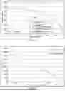
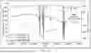
Liquid loading may be predicted at nominal wellhead pressure at the end of a well's life or production cycle. This may normally be measured as the minimum line pressure that the well can reach depending on the downstream surface network. Based on this future wellhead pressure (“WHP”), the corrected critical gas rate may be computed using the workflow described above (i.e., the onset point is denoted at 602 on the critical rate curve in FIG. 6). Based on nominal gas inflow performance curve parameters, the required average reservoir pressure to reach the onset point characterized by the nominal wellhead pressure and its corresponding corrected critical gas rate may be determined. In FIG. 6, this is denoted as the intersection of the critical gas rate curve 604 and the future IPR curve 606. In embodiments, a material balance may be used to estimate the required pressure depletion from current reservoir pressure and incremental cumulative gas production, as shown in FIG. 7. Based on an average rate of production between current condition and the onset point, the average time to liquid load may then be estimated. In embodiments, method steps for performing correction of the critical gas rate and/or determination of the onset point for liquid loading may include analysis of any other suitable measurements available to an operator and associated with the well. Further, any performance steps (i.e., determining, performing, identifying, calculating, etc.) provided herein may utilize any suitable measurements associated with the well.

Below, several case studies are presented as examples using the proposed LLPD workflow to calibrate critical gas rates and determine and/or predict liquid loading.

Example 1—Synthetic Benchmark

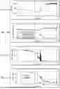
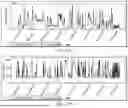
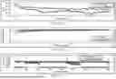
The first example involved using a commercial multiphase transient flow simulator to model a 10,000 ft vertical well producing dry gas and water. The well performed at a wellhead pressure of 100 psia with constant well productivity index, reservoir pressure, and water-gas ratio (WGR). The inflow gas velocity was controlled using reservoir pressure to mimic depletion over time. After 8 hours of initial flow, the inflow was reduced for 4 hours, resulting in low gas velocity that induces slugging. Eventually, this led to liquid loading, simulating the transition from stable annular flow to slugging and eventually bubble flow until the gas flow into the wellbore stopped. After about 8 hours of pressure recharge, the well was opened again, and the process repeated for a total of 4 cycles. The calculated bottomhole pressure, surface gas rate, surface water rate, downhole gas superficial velocity, and downhole water superficial velocity are shown in FIGS. 8A-8D.

This first example provides a comparison of the first, second, and third empirical correlations against the simulated liquid loading phenomenon. The onset of liquid loading may be characterized by the instability in gas rates and the sharp decline in production rate. The differential bottomhole gas and water velocity may result in significant liquid holdup that increases bottomhole pressure, reduces drawdown, and may shut down the well. For this vertical well, the critical rates determined by the second and third correlations are similar, while the critical rate determined by the first correlation provides a 20% higher estimate.

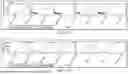
This first example may provide insights into the dynamic of liquid loading, as shown in FIGS. 9A-9E, which display the liquid volume fraction, referred to as “liquid holdup,” along the wellbore at three distinct time points: before liquid loading begins, at the onset of liquid loading (marked by a reduction in gas velocity (i.e., at bottom hole conditions) to critical velocity), and after liquid loading has commenced. With reference to FIGS. 8A-9E, all correlations provided estimates of critical rates higher than the observed outcomes. This may show the necessity of calibrating these correlations based on known onset points of liquid loading. This calibration process may ensure that empirical correlations accurately capture the dynamic conditions encountered in gas wells, leading to more dependable predictions. Ultimately, calibration based on known onset points may enhance the accuracy and applicability of critical rate calculations, thereby facilitating proactive management of liquid loading issues and optimization of production performance.

Example 2—Unconventional Gas Well-Over-Estimation of Critical Rate in a Stable Well

In the second example, a gas well from a major onshore unconventional basin in North America was utilized. The well had negligible condensate and WGR ranging from 0.208 to 0.286 STB/MSCF. By analyzing 14 days of production data and employing the LLDP methodology to assess liquid loading, no liquid loading events were observed. This conclusion is supported by the stable high-frequency rates and wellhead pressures, which do not indicate any instability induced by liquid loading, as shown in FIGS. 10A-10B.

However, with reference to FIG. 11, the first, second, and third empirical correlations over-estimated the critical rates incorrectly predicting liquid loading at least a few times during the period. Incidentally, the third correlation is the closest to the actual gas rate, and consequently during the calibration process it would have the least adjustment (i.e., α_j*=0.927), with the given knowledge that the well is not experiencing loading. In calibration, the critical rate may be adjusted to a level lower than the actual gas rate to indicate the absence of liquid loading.

Example 3—Unconventional Gas Well-Over-Estimation of Critical Rate in a Liquid Loaded Well

In the third example, another well from the same field as in Example 2 is considered here that had negligible condensate and WGR ranging from 0.250 to 0.330 STB/MSCF. By analyzing 14 days of production data and employing the LLDP methodology to assess liquid loading, several liquid loading events were observed, marked as vertical dotted lines in FIGS. 12A-12B. This observation may align with the instability evident in the wellhead pressures and gas rates throughout the entire 14-day period surrounding these events. As shown in FIG. 13, according to the identified liquid loading events, the first and second correlations tend to overestimate the critical rates, while the third correlation underestimates them. Notably, the second correlation appears to require the least adjustment (i.e., α_j*=0.886). Consequently, said second correlation was selected for tuning purposes to calculate the calibrated critical rate.

Example 4—Unconventional Gas Well-Optimizing Gas Lift Performance at Field Scale

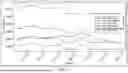
The fourth example was produced from a major unconventional basin in North America, and continuous gas lift injection was used to augment produced gas from the reservoir to lift the associated liquids. Using the LLDP method to calibrate critical rates for multiple wells, instructions for minimum gas injection rates tailored to individual wells have been determined with the objective of achieving stable operation devoid of interruptions due to liquid loading. This approach has yielded a notable decrease in instances of excessive gas injection in certain wells as compared to previous recommendations and/or instructions generated using the first correlation with a safety margin, which tended to overestimate critical rates and consequently led to excessive injection. Consequently, the optimization of gas lift performance at the field scale may reduce the operating cost associated with buy-back of lift gas through the utilization of calibrated critical rates. FIG. 14 illustrates the changes in gas lift operations at the field level over a 6-month implementation period, accompanied by corresponding formation gas production rates. Notably, this approach led to a 30% reduction in overall injection compared to the baseline at the beginning of the 6-month period, when such recommendations and/or instructions were not employed, highlighting its effectiveness in optimizing gas lift operations and maximizing production efficiency.

Example 5—Conventional Onshore Gas Field-Liquid Loading Detection and Well Cycling

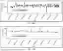
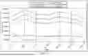
In the fifth example, an analysis focused on liquid loading detection and well cycling within a conventional gas field is presented which leverages actual high frequency data from mature onshore gas fields. FIGS. 15A-15B illustrate a set of plots of the measured high frequency gas rate and tubing pressure during a 7-day period, exhibiting a cyclic nature that is indicative of liquid loading and well cycling activities. Liquid loading events, as detected by the LLDP method, are denoted by the dotted lines. These events correspond to fluctuations in the actual gas rate and are corroborated by the wellhead pressure data, as shown in FIGS. 15A-15B.

The detected liquid loading events may be used to calibrate the empirical correlations for critical gas rate. This is illustrated in FIG. 16 where the first, second, and third correlations overestimate critical rates. The corrected critical rate based on the second correlation with a calibration factor of α_j*=0.381, aligns more closely with the nature of the liquid loading behavior observed, which may show a more accurate representation for the well cycling process. The corrected critical rate plot behaves in accordance with liquid loading nature of the well in contrast with the standard correlations that do not always conform to the detected events.

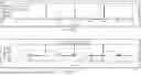
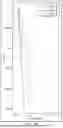
Example 6—Conventional Onshore Gas Field-Liquid Loading Detection Using Frequency Analysis

In the sixth example, frequency analysis was used to examine surface gas rate measurements from an onshore gas well. FIGS. 17A-17C illustrate a set of plots showing two distinct, 1-week flow periods from the well's history, where the well was initially flowing steady and subsequently under liquid loaded condition. The FIGS. 17A-17C provide that during stable flow, the energy of the signal is more evenly distributed at multiple scales of frequency. Consequently, the well may exhibit a more gradual, normalized cumulative power density curve. However, during liquid loading, there is a concentration of high energy at lower frequencies resulting in a steeper normalized cumulative power density. Correspondingly, the Gini coefficients from Equation 4 for the stable flow and liquid loaded periods are 0.039 and 0.105, respectively.

Example 7—Conventional Onshore Gas Field-Liquid Loading Prediction

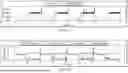
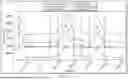
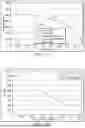
The seventh example provides that accurate prediction of liquid loading events is paramount for optimizing production from conventional gas fields. For example, all gas wells may eventually decline and predicting the onset of liquid loading may help with proactive planning of mitigation strategies and overall better field management. The LLDP method may integrate reservoir material balance (best seen in FIG. 18B) with nodal analysis (best seen in FIG. 18A) based on latest operating conditions using routinely collected production data.

With reference to FIGS. 18A-18B, the well's initial inflow performance curve (“IPR”) 1802 was estimated from measured surface rates and tubing pressure using automatic detection of stable flowing periods. When the operating point moves from right to the left of the critical rate curve 1804, the gas velocity may be expected to drop below critical velocity and trigger liquid loading. For a known minimum tubing pressure (i.e., abandonment pressure), by estimating the required pressure depletion for the IPR 1802 to intersect the critical rate curve 1804, it may be possible to forecast the incremental cumulative production before onset of liquid loading. For abandonment pressure of 50 psia, the estimated time to liquid load is predicted to be 122 days with 60 MMSCF cumulative gas production. This prediction model may be instrumental for operational planning, allowing for timely interventions such as well cycling, velocity strings, or other adjustments in production strategies.

The present disclosure provides systems and methods using a data-driven LLDP method to identify the onset of liquid loading. For example, there are limitations to existing empirical methods for accurately detecting liquid loading and estimating critical gas rate. To address these, the LLDP may leverage high frequency measurements (namely, gas rate and wellhead pressure) to detect physical flow instabilities associated with liquid loading to promptly detect its onset. Additionally, an optimization workflow to calibrate the critical rate using the nearest empirical correlation is proposed and used to align it with detected liquid loading flags, resulting in a refined critical rate estimation. Several field case studies were presented in Examples 1-7 to demonstrate the efficacy of the LLDP method in both conventional and unconventional wells, highlighting advancements in liquid loading detection and critical rate estimation. The improved critical rate estimation may assist in improved gas lift optimization and significant cost savings as demonstrated in one of the examples for unconventional gas field implementations. Further the present disclosure may provide how the calibrated critical rate can be integrated with nodal analysis and gas material balance to predict the timing of liquid loading onset and estimated recovery. This comprehensive approach may not only offer a robust methodology for characterizing liquid loading and extracting valuable insights but also may provide actionable recommendations for optimizing artificial lift operations and maximizing hydrocarbon recovery.

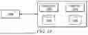
FIG. 19 illustrates a block diagram of an exemplary control unit 1900 in accordance with some embodiments of the present disclosure. In certain example embodiments, control unit 1900 may be configured to create and maintain one or more databases 1906 that include information concerning one or more reservoirs or reservoir models. In certain example embodiments, control unit 1900 is configured to use information from database(s) 1906 to train one or many machine learning algorithms, including, but not limited to, artificial neural network, random forest, gradient boosting, support vector machine, kernel density estimator, and any combination thereof. In some embodiments, control unit 1900 may include one more processors, such as processor 1902. Processor 1902 may include, for example, a microprocessor, microcontroller, digital signal processor (DSP), application specific integrated circuit (ASIC), or any other digital or analog circuitry configured to interpret and/or execute program instructions and/or process data. In some embodiments, processor 1902 may be communicatively coupled to memory 1904. Processor 1902 may be configured to interpret and/or execute non-transitory program instructions and/or data stored in memory 1904. Program instructions or data may constitute portions of software for carrying out estimations of reservoir or well performance characteristics, as described herein. Memory 1904 may include any system, device, or apparatus configured to hold and/or house one or more memory modules; for example, memory 1904 may include read-only memory, random access memory, solid state memory, or disk-based memory. Each memory module may include any system, device or apparatus configured to retain program instructions and/or data for a period of time (e.g., computer-readable non-transitory media).

Although control unit 1900 is illustrated as including two databases 1906, control unit 1900 may contain any suitable number of databases and machine learning algorithms. Control unit 1900 may be communicatively coupled to one or more displays 1908 such that information processed by control unit 1900 may be conveyed to operators at or near the well or may be displayed at a location offsite.

Modifications, additions, or omissions may be made to FIG. 19 without departing from the scope of the present disclosure. For example, FIG. 19 shows a particular configuration of components for control unit 1900. However, any suitable configurations of components may be used. For example, components of control unit 1900 may be implemented either as physical or logical components. Furthermore, in some embodiments, functionality associated with components of control unit 1900 may be implemented in special purpose circuits or components. In other embodiments, functionality associated with components of control unit 1900 may be implemented in a general purpose circuit or components of a general purpose circuit. For example, components of control unit 1900 may be implemented by computer program instructions.

Modifications, additions, or omissions may be made to the systems and apparatuses described herein without departing from the scope of the disclosure. The components of the systems and apparatuses may be integrated or separated. Moreover, the operations of the systems and apparatuses may be performed by more, fewer, or other components. Additionally, operations of the systems and apparatuses may be performed using any suitable logic comprising software, hardware, and/or other logic. As used in this document, “each” refers to each member of a set or each member of a subset of a set.

Modifications, additions, or omissions may be made to the methods described herein without departing from the scope of the invention. For example, the steps may be combined, modified, or deleted where appropriate, and additional steps may be added. Additionally, the steps may be performed in any suitable order without departing from the scope of the present disclosure.

Although the present invention has been described with several embodiments, a myriad of changes, variations, alterations, transformations, and modifications may be suggested to one skilled in the art, and it is intended that the present invention encompass such changes, variations, alterations, transformations, and modifications as fall within the scope of the appended claims. Therefore, the present invention is well adapted to attain the ends and advantages mentioned as well as those that are inherent therein. The particular embodiments disclosed above are illustrative only, as the present invention may be modified and practiced in different but equivalent manners apparent to those skilled in the art having the benefit of the teachings herein. Furthermore, no limitations are intended to the details of construction or design herein shown, other than as described in the claims below. It is therefore evident that the particular illustrative embodiments disclosed above may be altered or modified and all such variations are considered within the scope and spirit of the present invention. Also, the terms in the claims have their plain, ordinary meaning unless otherwise explicitly and clearly defined by the patentee. The indefinite articles “a” or “an,” as used in the claims, are each defined herein to mean one or more than one of the element that it introduces.

A number of examples have been described. Nevertheless, it will be understood that various modifications can be made. Accordingly, other implementations are within the scope of the following claims.