AXIAL COILS BASED QUANTITATIVE EVALUATION OF TOOL AND PIPE ECCENTERINGS

Description

CROSS-REFERENCE TO RELATED APPLICATIONS

This application is a Non-Provisional Application claiming priority to U.S. Provisional Patent Application No. 63/737,090, entitled “AXIAL COILS BASED QUANTITATIVE EVALUATION OF TOOL AND PIPE ECCENTERINGS IN UP TO 5-PIPES COMPLETION WELLS”, filed Dec. 20, 2024, which is herein incorporated by reference.

BACKGROUND

The subject matter disclosed herein relates to systems and methods to increase efficiencies during pipe inspections.

This section is intended to introduce the reader to various aspects of art that may be related to various aspects of the present techniques, which are described and/or claimed below. This discussion is believed to be helpful in providing the reader with background information to facilitate a better understanding of the various aspects of the present disclosure. Accordingly, it should be understood that these statements are to be read in this light, and not as admissions of prior art.

The relative positioning of pipes within a wellbore provides critical information for well integrity evaluation, particularly information about potential cementing, bonding and pipe corrosion issues, as well as drilling holes in the pipes for sidetracking existing wells. Accurate measurements of the positioning of the pipes can be useful, for example, when drilling sidetrack wells, when sealing (i.e., decommissioning) a well, and/or in other situations. Misaligned pipes within the wellbore can cause issues in obtaining a proper seal as part of decommissioning a well, drilling a sidetrack well, etc. Accordingly, it would be beneficial to provide accurate measurements of quantitative positioning of each of the pipes in a wellbore.

BRIEF DESCRIPTION OF THE DRAWINGS

Various aspects of this disclosure may be better understood upon reading the following detailed description and upon reference to the drawings in which:

FIG. 1 depicts an example wellsite system that can utilize various downhole tools and surface tools, in accordance with embodiments of the present disclosure;

FIG. 2 depicts a well control system and data acquisition tool that operate in conjunction with the wellsite system of FIG. 1 in conjunction with natural resource operations, in accordance with embodiments of the present disclosure;

FIG. 3 depicts an example of the data acquisition tool of FIG. 2, in accordance with embodiments of the present disclosure;

FIG. 4 illustrates an example of the data acquisition tool of FIG. 3 disposed in a pipe, in accordance with embodiments of the present disclosure;

FIG. 5 depicts a first example of graphs illustrating measurement of voltages in two concentric pipes to determine offset between the pipes via the data acquisition tool of FIG. 3, in accordance with embodiments of the present disclosure;

FIG. 6 depicts a second example of graphs illustrating measurement of voltages in five concentric pipes to determine offset between the pipes via the data acquisition tool of FIG. 3, in accordance with embodiments of the present disclosure;

FIG. 7 depicts a third example of graphs illustrating measurement of voltages in five concentric pipes to determine offset between the pipes via a data acquisition tool of FIG. 2, in accordance with embodiments of the present disclosure; and

FIG. 8 depicts a flow chart describing a technique for determining an offset between concentric pipes, in accordance with embodiments of the present disclosure.

DETAILED DESCRIPTION OF SPECIFIC EMBODIMENTS

One or more specific embodiments will be described below. In an effort to provide a concise description of these embodiments, not all features of an actual implementation are described in the specification. It should be appreciated that in the development of any such actual implementation, as in any engineering or design project, numerous implementation-specific decisions must be made to achieve the developers' specific goals, such as compliance with system-related and business-related constraints, which may vary from one implementation to another. Moreover, it should be appreciated that such a development effort might be complex and time consuming, but would nevertheless be a routine undertaking of design, fabrication, and manufacture for those of ordinary skill having the benefit of this disclosure.

Embodiments of the present disclosure may direct towards an electromagnetic model for enabling sensitivity-based selection of tool channels to excite and measure the correct tool channels. The relative positioning of the pipes inside a wellbore provides useful information about potential cementing, bonding and pipe corrosion issues, as well as drilling holes in the pipes for sidetracking existing wells. Present embodiments include development and implementation of a data acquisition tool that is programmable to excite and measure signals at receivers each having respective sensitivity to one or more pipes so as to allow for measurement of the respective locations of the one or more pipes with respect to an axis (e.g., an axis passing vertically through the data acquisition tool with respect to the surface) as a eccentering value. Embodiments additionally include implementation of a system that provides sensitivity based selection of tool channels which can be inverted for quantitative positioning of each pipe of a set of one or more pipes in a borehole. This sensitivity based channel selection can be implemented in conjunction with a disentangling-based inversion scheme to generate quantitative casing positions (i.e., positions of the one or more pipes with respect to the data acquisition tool).

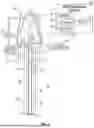
With the foregoing in mind, FIG. 1 illustrates a drilling system 10 that may employ the systems and methods of this disclosure. The drilling system 10 may be used to drill a borehole 12 into a geological region 14. In the drilling system 10, a drilling rig 18 may rotate a drill string 20 within the borehole 12. As the drill string 20 is rotated, a drilling fluid pump 22 may be used to pump drilling fluid, which may be referred to as “mud” or “drilling mud,” downward through the center of the drill string 20, and back up around the drill string 20. At the surface, return drilling fluid may be filtered and conveyed back to a mud pit 24 for reuse. The drilling fluid may travel down to the bottom of the drill string 20 known as the bottom-hole assembly (BHA) 26. The drilling fluid may be used to rotate, cool, and/or lubricate a drill bit 28 that may be a part of the BHA 26. The fluid may exit the drill string 20 through the drill bit 28 and carry drill cuttings away from the bottom of the borehole 12 back to the surface.

Additionally illustrated in FIG. 1 is a series of concentric pipes or casings that are installed about the borehole 12. These casings can be made of metal, such as steel, and when installed about the borehole 12, represent a wellbore that operates to prevent collapse of the borehole 12. In this way, the casings operate to provide structural support to the borehole 12 and the casings can be cemented in place to provide the structural support to the borehole 12. An uppermost casing can be the conductor casing 30. The conductor casing 30 can be approximately, for example, 60 ft long and can operate as a mount which a casing head is installed. The conductor casing 30 can be cemented to surface.

The casings of the wellbore can additionally include a surface casing 32. The surface casing 32 can be approximately, for example, 1000 ft-3000 ft long and can operate to, for example, isolate the borehole 12 from the subsurface regions about the borehole 12. In some embodiments, the surface casing 32 is additionally cemented to surface. The casings of the wellbore can further include an intermediate casing 34 (or multiple intermediate casings 34). The intermediate casing 34 can operate to isolate zones of the formation into which the borehole 12 is drilled and the intermediate casing 34 can include a cement top that operates to isolate any hydrocarbon zones. Some wells include multiple intermediate casings 34, however, other wells can omit the intermediate casing 34. The intermediate casing 34 can be secured with cement to provide stability to the wellbore.

A production casing 36 is additionally illustrated in FIG. 1. The production casing 36 can operate to isolate production zones and contain formation pressures and the production casing 36 is also cemented to reduce movement of the production casing from its installed position. As illustrated, the conductor casing 30, the surface casing 32, the one or more intermediate casings 34, and the production casing 36 are concentrically positioned with the conductor casing 30 (the outermost casing) having the greatest diameter, the surface casing 32 (the second outermost casing) having a reduced diameter with respect to the conductor casing 30, the one or more intermediate casings 34 (the third and additional outermost casings) having reduced diameters with respect to one another and to the surface casing 32, and the production casing 36 (the innermost casing) having a reduced diameter with respect to the one or more intermediate casings 34.

As additionally illustrated, the BHA 26 may include one or more logging tools 38. The BHA 26 may thus convey the one or more logging tools 38 through the geological region 14 via the borehole 12. In other embodiments, the BHA 26 can be removed and in its place a data acquisition tool may be conveyed through the geological region 14 via the borehole 12. As described in greater detail herein, the one or more logging tools 38 and the data acquisition tool (referred to herein collectively as downhole tools) may be any suitable downhole tool that emits electromagnetic waves within the borehole 12 (e.g., a downhole environment). The downhole tools may collect a variety of information relating to the geological region 14, the state of drilling in the borehole 12, and/or the state of the casings, depending on the downhole tool that is deployed. In some embodiments, the one or more logging tools 38 may be logging-while drilling (LWD) tools that measure physical properties of the geological region 14, such as density, porosity, resistivity, lithology, and so forth. Likewise, the one or more logging tools 38 may be measurement-while-drilling (MWD) tools that measure certain drilling parameters, such as the temperature, pressure, orientation of the drill bit 28, mapping-while-drilling tools, and so forth. Moreover, the data acquisition tool can operate to measure attributes of the casings, for example, integrity of the casings. In other embodiments, as discussed in greater detail herein, the data acquisition tool can operate to measure eccentering of the casings (i.e., determination and/or measurement of the respective locations of the casings with respect to an axis passing vertically through the data acquisition tool with respect to the surface) to determine misalignment of the casings.

The one or more downhole tools may receive energy from an electrical energy device or an electrical energy storage device, such as an auxiliary power source 40 or another electrical energy source to power the tool. In some embodiments, the one or more one or more downhole tools may include a power source within the one or more downhole tools, such as a battery system or a capacitor, to store sufficient electrical energy to emit and/or receive electromagnetic waves.

Communications 42, such as control signals, may be transmitted from a data processing system 44 (processing system 44) to the one or more downhole tools and communications 42, such as data signals related to the results/measurements of the one or more downhole tools, may be returned to the data processing system 44 from the one or more downhole tools. The data processing system 44 may be any electronic data processing system that can be used to carry out the systems and methods of this disclosure. For example, the data processing system 44 may include one or more processors 46, which may execute instructions stored in memory 48 and/or storage 50. The memory 48 and/or the storage 50 of the data processing system 44 may be any suitable article of manufacture that can store the instructions. In certain embodiments, the one or more processors 46 may include a microprocessor, a microcontroller, a processor module or subsystem, a programmable integrated circuit, a programmable gate array, a digital signal processor (DSP), or another control or computing device. In certain embodiments, the one or more processors 46 may include machine learning (ML) and/or artificial intelligence (AI) based processors. Likewise, the one or more processors 46 may operate to implement a trained ML model as part of an AI processing system.

In certain embodiments, the memory 48 and storage 50 are implemented as one or more non-transitory computer-readable or machine-readable storage media. In certain embodiments, the memory 48 may include one or more different forms of memory, including semiconductor memory devices, such as dynamic or static random access memories (DRAMs or SRAMs), erasable and programmable read-only memories (EPROMs), electrically erasable and programmable read-only memories (EEPROMs) and flash memories. The storage 50 may include solid state drives, magnetic disks such as fixed, floppy and removable disks; other magnetic media including tape; optical media such as compact disks (CDs) or digital video disks (DVDs); or other types of storage devices. Note that the computer-executable instructions and associated data of the analysis module(s) may be provided on one computer-readable or machine-readable storage medium of the memory 48 or the storage 50, or alternatively, may be provided on multiple computer-readable or machine-readable storage media distributed in a large system having possibly plural nodes. Such computer-readable or machine-readable storage medium or media are considered to be part of an article (or article of manufacture), which may refer to any manufactured single component or multiple components. In certain embodiments, the storage 50 may be located either in the machine running the machine-readable instructions or may be located at a remote site from which machine-readable instructions may be downloaded over a network for execution.

As illustrated, the data processing system 44 may optionally also include a display 52, which may be any suitable electronic display, and may display images generated by the processor 46. The data processing system 44 may be a local component of the drilling system 10 (i.e., at the surface), within the one or more downhole tools (i.e., downhole), a device located proximate to the drilling operation, and/or a remote data processing device located away from the drilling system 10 to process downhole measurements in real time or sometime after the data has been collected. In some embodiments, the data processing system 44 may be a portable computing device (e.g., tablet, smart phone, or laptop) or a server remote from the drilling system 10. In some embodiments, the one or more downhole tools may store and process collected data in the downhole tool or send the data to the surface for processing via communications 42 described above, including any suitable telemetry (e.g., electrical signals pulsed through the geological region 14 or mud pulse telemetry using the drilling fluid).

In one embodiment, one or more operations may be controlled by a processor 46 of the data processing system 44. For example, FIG. 2 illustrates a block diagram of the data processing system 44 that is communicatively coupled to one or more data acquisition tools 54. In the illustrated embodiment, a data acquisition tool 54 includes processing circuitry 56, memory 58, an acquisition system 60, and storage 62. In some embodiments, the processing circuitry 56 may include an ASIC (application specific integrated circuit), field programmable gate array (FPGA), a micro control unit (MCU), a digital signal processor (DSP), and the like. In some embodiments, the data acquisition tool 54 communicates with the data processing system 44 via a data cable 64, telemeter, or other suitable techniques. For example, the data acquisition tool 54 may communicate measurements obtained by a one or more sensors (or receivers) as part of the acquisition system 60. In turn, a processor 46 of the surface control system (e.g., data processing system 44) may determine certain parameters (e.g., casing integrity, casing eccentering, and so forth) based on the measurements. In such embodiments, the acquisition system 60 may include an emission source (e.g., an antenna) as well as one or more receivers to acquire, obtain, or otherwise measure measurements, for example, as part of eddy based current based pipe inspection.

FIG. 3 illustrates an example of a data acquisition tool 54 (e.g., a non-co-located axial coil-based measuring tool) that can be utilized in an Eddy current based pipe inspection operation to determine pipe (e.g., casing) eccentering. The data acquisition tool 54, as illustrated, includes one or more coils (e.g., co-axial coils) as a transmitter 66 (e.g., T) as well as receiver 68 (e.g., R1), receiver 70 (e.g., R2), receiver 72 (e.g., R3), receiver 74 (e.g., R4), receiver 76 (e.g., R5), receiver 78 (e.g., R6), and receiver 80 (e.g., R7) disposed along the data acquisition tool 54. One or more of the receivers 68-80 can include, for example, tilted coils and/or transverse coils and/or axial coils. Moreover, while seven receivers 68-80 are illustrated, it should be appreciated that more or fewer receivers can be present in the data acquisition tool 54.

In some embodiments, the transmitter 66 of the data acquisition tool 54 consists of a single exciting axial coil as transmitter 66 (T) and multiple axial receiver coils as receivers 68-80 (R1-R7) whereby the receivers 68-80 (R1-R7) are each respectively positioned at different axial distances from transmitter (T). The transmitter 66 (T) can be excited, for example, by a time-domain pulse or a series of continuous wave (CW) multifrequency excitations. The time-domain pulse excitation primarily facilitates collocated sensor acquisition during an off cycle but also suffices to record non-collocated responses, which can electronically be converted into multi-frequency (harmonics) measurements. However, the decreasing signal to noise ratio of higher harmonics due to the inverse scaling with frequency can be addressed by CW excitation where each frequency is excited individually to achieve maximum signal-to-noise ratio. In some embodiments, the fundamental frequency of the tool can from approximately, for example, as low as 0.3 Hz to penetrate multiple metallic casings (e.g., three, four, five, or more casings).

FIG. 4 shows a diagram 82 illustrating the data acquisition tool 54 operating while disposed in a pipe, for example, production casing 36. As illustrated, the production casing 36 includes a tube wall 84 as a metal cylinder or annulus surrounding the data acquisition tool 54. The outer diameter 86 of the production casing 36 includes the tube wall 84 of the production casing 36 as well as center region of the production casing 36 having an inner diameter 88 less than the outer diameter 86 of the production casing (i.e., the inner diameter 88 can be equal to the outer diameter 86 minus a diameter of the tube wall 84). The data acquisition tool 54 can be selected to fit within the inner diameter 88 of the production casing 36.

As illustrated, the data acquisition tool 54 includes transmitter 66 (e.g., T) as well as receiver 68 (e.g., R1) disposed at a distance 90 from one another. It should be noted that only receiver 68 is (e.g., R1) is illustrated, but one or more additional receivers (e.g., receivers 70-80 as R2-R7) can be part of the data acquisition tool 54. However, for purposes of discussion, the underlying physics of inspecting metallic tubes using eddy-current techniques are discussed using transmitter 66 (e.g., T) and receiver 68 (e.g., R1) of the data acquisition tool 54. In some embodiments, for each excitation frequency (i.e., a rate at which a time-varying magnetic field oscillates), the transmitter 66 (e.g., T), for example, as an exciter coil, generates a magnetic field which is distributed in space, including through the inner diameter 88 and into the tube wall 84 of the production casing 36. The magnetic field generated by the transmitter 66 (e.g., T) is illustrated as including a direct coupling field 92 as a portion of the magnetic field that can be measured by the receiver 68 (e.g., R1) as well as an indirect coupling field 94 as a portion of the magnetic field that can be measured by the receiver 68.

When the transmitter 66 (e.g., T) generates a magnetic field at an excitation frequency, this induces eddy currents (i.e., induced currents generated in response to a changing magnetic field) in the surrounding pipes (including production casing 36). The eddy currents are dominated by direct coupling in the direct coupling zone 96 (i.e., the region of the tube wall 84 adjacent to the transmitter 66, which may also be referred to as the near field zone), the eddy currents match and cancel in the transition zone 98 (i.e., the region of the tube wall 84 disposed generally between the transmitter 66 and the receiver 68), and the eddy currents are dominated in the remote field zone 100 (i.e., the region of the tube wall 84 adjacent to the receiver 68, which may also be referred to as the far field zone or the indirect coupling zone). In some embodiments, the far field zone 100 can be disposed at, for example, approximately twice or three times the outer diameter of the largest pipe being inspected. As evident in FIG. 4, the direct coupling field 92 and the secondary (“indirect” or induced) couplings (e.g., the indirect coupling field 94) compete in the coil region of the transmitter 66 for each frequency generated by the transmitter 66, which results in a distribution of fields which can be grouped into the direct coupling zone 96, the transition zone 98, and the remote field zone 100.

In the remote field zone 100, typically at spacings of approximately, for example, two to three times the outer diameter of the largest pipe being inspected, the induced secondary field (i.e., indirect coupling field 94) is stronger as the primary magnetic field (i.e., direct coupling field 92) drops off at a rate of 1/R3, where R is a measured distance from the coil of the transmitter 66. Additionally, as the distance spacing increases, ohmic losses incurred in the induced current along the pipe length are less than the cubic reduction in direct coupling fields. It is in the remote field zone 100 that a remote field eddy current, is generated and can be measured, for example, to determine and/or evaluate total metal thickness.

In the direct coupling zone 96, the primary magnetic field (i.e., the direct coupling field 92) is dominant due to the small R compared to the secondary field (i.e., indirect coupling field 94), which suffers from exponential decay while inducing currents in metallic pipes. In the transition zone 100 (i.e., the intermediate region between the direct coupling zone 96 and the remote field zone 100), neither of the primary magnetic field (i.e., the direct coupling field 92) nor the secondary field (i.e., indirect coupling field 94) dominates the other. This results from each of the primary magnetic field (i.e., the direct coupling field 92) and the secondary field (i.e., indirect coupling field 94) having approximately the same order of magnitudes but opposite directions (e.g., due to Faraday's and Lorentz's Law).

In some embodiments, the direct coupling zone 96 is predominantly sensitive to the relative position of the data acquisition tool 54 inside a first pipe (e.g., production casing 36) and the inner surface of the first pipe (e.g., production casing 36). The transition zone 98, in contrast, represents the region where the eccentering beyond the first pipe (e.g., the production casing 36) becomes more prevalent. Accordingly, the transition region 98 is the region where the maximum sensitivity to pipe eccentering can be targeted to be extracted and exploited in conjunction with present embodiments. In some embodiments, the spacings of interest (e.g., as part of the transition region) may be, for example, approximately values selected between 2-40 in. from the closest edge of the coil of the transmitter 66 with respect to the respective receivers (e.g., one or more of receivers 68-80 as R1-R7).

As previously discussed, the data acquisition tool 54 can operate to measure eccentering of the concentric pipes (e.g., one or more casings that can include the conductor casing 30, the surface casing 32, one or more intermediate casings 34, and/or the production casing 36). Measurement of eccentering of these concentric pipes (e.g., casings) can include the determination and/or measurement of the respective locations of the casings with respect to an axis passing vertically through the data acquisition tool with respect to the surface. This determined value of the locations of the one or more concentric pipes can be used to determine misalignment of the casings. In some embodiments, this misalignment information is used in cementing operation (e.g., when sealing or decommissioning a well), in drilling holes in the casings at a desired location as part of sidetracking operations to generate a new well extending from an existing well, and/or in other operations (for example, determining corrosion of the casings).

As part of a sidetracking operation, a cutting tool is placed in the wellbore to cut holes at a desired location from which a new well is to be drilled. However, if the concentric pipes are misaligned, a cutting tool of a particular size may not be able to extend sufficiently to cut through additional casings surrounding, for example, the production casing 36. This can lead to additional downtime as the smaller cutting tool is extracted and a larger cutting tool is run into the wellbore to complete a cut through the concentric pipes.

Similarly, if a well is to be sealed or decommissioned, misalignment of casings of the wellbore can lead to gaps between the casings, damage to the cement used in the wellbore, etc. To complete a decommissioning operation, determination of any misalignment of the casings (i.e., eccentering of the pipes) aids in determining if the wellbore is properly sealed and/or what steps can be taken to properly seal the well. Likewise, eccentering of casings provides an indication that corrosion of the pipes used as the casings are degrading, corroding, etc. In this manner, determination of eccentering of the casings can be useful in determining when and if casings are to be replaced and/or repaired.

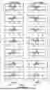
FIG. 5 depicts a first example of graphs illustrating measurement of voltages in two concentric pipes (e.g., an intermediate casing 34 and the production casing 36) to determine offset between the pipes utilizing the data acquisition tool 54. The processing circuitry 56 of the data acquisition tool 54 can operate to control the transmitter 66. In some embodiments, the transmitter 66 can be controlled to generate a series of continuous wave (CW) multifrequency excitations. That is, the transmitter 66 generates a continuous series of excitation frequencies as rates at which a time-varying magnetic field oscillates as generated by an exciter coil of the transmitter 66. Graph 102 of FIG. 5 corresponds to receiver 68 (R1) and the frequencies of the CW multifrequency excitations generated by the transmitter 66 are illustrated along the x-axis of graph 102. Resulting changes in voltages generated in casing 1 (e.g., production casing 36) due to the eddy currents generated in casing 1 in response to the CW multifrequency excitations are illustrated in as a change in voltage along the y-axis of graph 102.

Graph 102 additionally includes examples of changes in the generated voltages that correspond to different amounts of decentralization with respect to casing 1 (e.g., production casing 36). For example, when there is no decentralization, no change in response is registered as illustrated by result 104. This corresponds to 0% eccentering value (i.e., no decentering of casing 1 with respect to an axis passing vertically through the data acquisition tool 54 with respect to the surface). Likewise, when maximum decentralization has occurred (e.g., when the outer diameter of the inner pipe, casing 1, is contacting the inner diameter of the outer pipe, casing 2), a corresponding 100% eccentering value is registered. This 100% eccentering value is illustrated as a voltage having a real component 106 and an imaginary component 108. If, instead, decentralization at a level of 75% of maximum decentralization has occurred a corresponding 75% eccentering value is registered. This 75% eccentering value is illustrated as a voltage having a real component 110 and an imaginary component 112. If decentralization at a level of 50% of maximum decentralization has occurred, a corresponding 50% eccentering value is registered, which is illustrated as a voltage having a real component 114 and an imaginary component 116. If decentralization at a level of 25% of maximum decentralization has occurred, a corresponding 25% eccentering value is registered, which is illustrated as a voltage having a real component 118 and an imaginary component 120. It should be noted that only one eccentering value will be generated and it can correspond to one of the above noted eccentering values or another value between 0-100%.

FIG. 5 additionally illustrates graph 122 that corresponds to receiver 70 (R2) and the frequencies of the CW multifrequency excitations generated by the transmitter 66 are illustrated along the x-axis of graph 122. Resulting changes in voltages generated in casing 1 (e.g., production casing 36) due to the eddy currents generated in casing 1 in response to the CW multifrequency excitations are illustrated in as a change in voltage along the y-axis of graph 122. Similarly, graph 124 corresponds to receiver 72 (R3), graph 126 corresponds to receiver 74 (R4), graph 128 corresponds to receiver 76 (R5), graph 130 corresponds to receiver 78 (R6), and graph 132 corresponds to receiver 80 (R7). In each of graphs 122-132, the frequencies of the CW multifrequency excitations generated by the transmitter 66 are illustrated along the x-axis of the corresponding graph. Resulting changes in voltages generated in casing 1 (e.g., production casing 36) due to the eddy currents generated in casing 1 in response to the CW multifrequency excitations are likewise illustrated in as a change in voltage along the y-axis of the corresponding graph.

It should be noted that the y-axis for each of graphs 102 and graphs 122-132 differ from one another. Indeed, this can represent that the change in voltage corresponding to casing 1 (e.g., production casing 36) can be determined using the measurements from R1, corresponding to graph 102. The change in voltage represented in graphs 122-132 may be outside of the measurement capabilities of receivers 72-80. Accordingly, the eccentering of casing 1 can be determined using the measured voltages from receiver 68 (R1).

FIG. 5 additionally illustrates graph 134 that corresponds to receiver 68 (R1) and the frequencies of the CW multifrequency excitations generated by the transmitter 66 are illustrated along the x-axis of graph 134. Resulting changes in voltages generated in casing 2 (e.g., intermediate casing 34) due to the eddy currents generated in casing 2 in response to the CW multifrequency excitations are illustrated in as a change in voltage along the y-axis of graph 134.

Graph 134 additionally includes examples of changes in the generated voltages that correspond to different amounts of decentralization with respect to casing 2 (e.g., intermediate casing 34). For example, when there is no decentralization, no change in response is registered as illustrated by result 136. This corresponds to 0% eccentering value (i.e., no decentering of casing 2 with respect to an axis passing vertically through the data acquisition tool 54 with respect to the surface). Likewise, when maximum decentralization has occurred (e.g., when the outer diameter of the inner pipe, casing 2, is contacting the inner diameter of the outer pipe, casing 3), a corresponding 100% eccentering value is registered. This 100% eccentering value is illustrated as a voltage having a real component 138 and an imaginary component 140. If, instead, decentralization at a level of 75% of maximum decentralization has occurred a corresponding 75% eccentering value is registered. This 75% eccentering value is illustrated as a voltage having a real component 142 and an imaginary component 144. If decentralization at a level of 50% of maximum decentralization has occurred, a corresponding 50% eccentering value is registered, which is illustrated as a voltage having a real component 146 and an imaginary component 148. If decentralization at a level of 25% of maximum decentralization has occurred, a corresponding 25% eccentering value is registered, which is illustrated as a voltage having a real component 150 and an imaginary component 152. It should be noted that only one eccentering value will be generated and it can correspond to one of the above noted eccentering values or another value between 0-100%.

FIG. 5 additionally illustrates graph 154 that corresponds to receiver 70 (R2) and the frequencies of the CW multifrequency excitations generated by the transmitter 66 are illustrated along the x-axis of graph 154. Resulting changes in voltages generated in casing 3 (e.g., intermediate casing 34) due to the eddy currents generated in casing 2 in response to the CW multifrequency excitations are illustrated in as a change in voltage along the y-axis of graph 154. Similarly, graph 156 corresponds to receiver 72 (R3), graph 158 corresponds to receiver 74 (R4), graph 160 corresponds to receiver 76 (R5), graph 162 corresponds to receiver 78 (R6), and graph 164 corresponds to receiver 80 (R7). In each of graphs 154-164, the frequencies of the CW multifrequency excitations generated by the transmitter 66 are illustrated along the x-axis of the corresponding graph. Resulting changes in voltages generated in casing 2 (e.g., intermediate casing 34) due to the eddy currents generated in casing 2 in response to the CW multifrequency excitations are likewise illustrated in as a change in voltage along the y-axis of the corresponding graph.

It should be noted that the y-axis for each of graphs 134 and graphs 154-164 differ. Indeed, this can represent that the change in voltage corresponding to casing 2 (e.g., intermediate casing 34) can be determined using the measurements from receiver 76 (R5) and receiver 80 (R7), corresponding to graph 160 and graph 164. The change in voltage represented in graph 134, graph 154, graph 156, graph 158, and graph 162 may be outside of the measurement capabilities of corresponding receiver 68, 70, 72, 74, and 78. Accordingly, the eccentering of casing 2 can be determined using the measured voltages from receiver 76 (R5) and receiver 80 (R7).

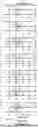
FIG. 6 illustrates a second example of graphs illustrating measurement of voltages in five concentric pipes (e.g., the production casing 36 as casing 1, an intermediate casing as casing 2, a second intermediate casing as casing 3, the surface casing as casing 4, and the conductor casing 30 as casing 5). Similar to the discussion above with respect to FIG. 5, the processing circuitry 56 of the data acquisition tool 54 can operate to control the transmitter 66. In some embodiments, the transmitter 66 can be controlled to generate a series of continuous wave (CW) multifrequency excitations. That is, the transmitter 66 generates a continuous series of excitation frequencies as rates at which a time-varying magnetic field oscillates as generated by an exciter coil of the transmitter 66. The graphs in row 166 correspond to receiver 68 (R1), the graphs in row 168 correspond to receiver 70 (R2), the graphs in row 170 correspond to receiver 72 (R3), the graphs in row 172 correspond to receiver 74 (R4), the graphs in row 174 correspond to receiver 76 (R5), the graphs in row 176 correspond to receiver 78 (R6), and the graphs in row 178 correspond to receiver 80 (R7). The frequencies of the CW multifrequency excitations generated by the transmitter 66 are illustrated along the x-axis of the graphs in rows 166-178. Resulting changes in voltages generated due to the eddy currents generated in response to the CW multifrequency excitations are illustrated in as a change in voltage along the y-axis of the graphs in rows 166-178.

The graphs of FIG. 6 are additionally illustrated as each being in column 180, column 182, column 184, column 186, or column 188. Column 180 corresponds to eccentering readings of casing 1, column 182 corresponds to eccentering readings of casing 2, column 184 corresponds to eccentering readings of casing 3, column 186 corresponds to eccentering readings of casing 4, and column 188 corresponds to eccentering readings of casing 5. Similar to discussed above with respect to FIG. 5, the y-axis of the graphs of FIG. 6 differ, reflecting capabilities of the respective receivers 68-80 to measure changes in voltage. For example, receiver 68 (R1) may be used to measure eccentering in casing 1. Receiver 76 (R5) and receiver 80 (R7) may be used to measure eccentering in casing 2. Receivers 70-80 (R2-R7) may be used to measure eccentering in casing 3. Receiver 78 (R6) and receiver 80 (R7) may be used to measure eccentering in casing 4 and casing 5. Each of the receivers noted above operates to measure voltages within the capability of the downhole receiver tool 54.

FIGS. 5 and 6 show the sensitivity of a representative downhole acquisition tool 54 to each of two and five pipe eccenterings (swept from centered (0%) to a possible extent in the radial direction (100%)). The change in responses compared to centered responses are shown with real and imaginary part of the voltages. Qualitatively, the changes in responses for the two and five pipe completions may look similar, but as the number of pipes change, the inner pipe responses also shift in frequency. Hence, in some embodiments, the sensitivity may be plotted for all completions of up to five pipes to show the relative strength of sensitivity, as well as to emphasize the relative shift in the peak of sensitivity with respect to frequency for each of the axial receiving spacings.

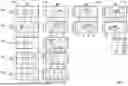
FIGS. 5 and 6 represented transmissions by a downhole acquisition tool 54 in which a transmitter 66 generated a series of CW multifrequency excitations. However, in other embodiments, the data acquisition tool 54 operates to excite the transmitter 66 as one or more time-domain pulses (i.e., at particular frequencies). FIG. 7 illustrates an example of graphs illustrating measurement of voltages in five concentric pipes to determine offset between the pipes via the data acquisition tool 54 operating using time-domain pulse excitations.

Similar to the discussion above with respect to FIGS. 5 and 6, the processing circuitry 56 of the data acquisition tool 54 can operate to control the transmitter 66 to generate the graphs in FIG. 7. In some embodiments, the transmitter 66 can be controlled to generate excitations at predetermined frequencies. That is, the transmitter 66 generates excitation frequencies at which a time-varying magnetic field oscillates as generated by an exciter coil of the transmitter 66. The graphs in row 190 correspond to a first excitation frequency (F1) at which the transmitter 66 generates a time-varying magnetic field. The graphs in row 192 correspond to a second excitation frequency (F2) at which the transmitter 66 generates a time-varying magnetic field. The graphs in row 194 correspond to a third excitation frequency (F3) at which the transmitter 66 generates a time-varying magnetic field. The graphs in row 196 correspond to a fourth excitation frequency (F4) at which the transmitter 66 generates a time-varying magnetic field. The graphs in row 198 correspond to a fifth excitation frequency (F5) at which the transmitter 66 generates a time-varying magnetic field.

Likewise, the graphs in column 200 correspond to a first receiver, for example receiver 68 (R1). The graphs in column 202 correspond to a second receiver, for example, receiver 70 (R2). The graphs in column 204 correspond to a third receiver, for example, receiver 72 (R3). The graphs in column 206 correspond to a fourth receiver, for example, receiver 74 (R4). Only four receivers are illustrated to show that the downhole acquisition tool 54 can operate with less than (or more than) seven receivers. Additionally, the locations of the first receiver, the second receiver, the third receiver, and the fourth receiver utilized in connection with FIG. 7 need not correspond to any of the receivers 68-80 illustrated in FIG. 3.

FIG. 7 illustrates graphs with results plotted in a phase (in degrees along the x-axis) vs. attenuation (in decibels along the y-axis) plot where different spacings of the receivers are represented by columns 200-206 while the frequencies increase from row 190 to row 198. The most useful channels are blown out to show separation of individual pipe responses, which may be sequentially extracted from the highest and shallowest channels for the first pipe, higher frequency and intermediate spacing for the second pipe, and medium and intermediate spacing for the third pipe, while phase sign switching in longer and deghosting coils for separation of eccentering in the fourth pipe and the fifth pipe. Thus, in operation, transmitting at frequency F5 will result in eccentering measurements for casing 1 and casing 2, transmitting at frequency F3 will result in eccentering measurements for casing 3, and transmitting at frequency F2 will result in eccentering measurements for casing 4 and casing 5. Additionally, it should be noted that for any graph, only one circle representative of an eccentering value for a particular casing will be present (although multiple values are illustrated in FIG. 7 for ease of understanding by the reader as to the types of eccentering values that can be generated).

FIG. 8 depicts a flow chart 208 describing a technique for determining an offset between concentric pipes. In block, pre-job sensitivity analysis and casing channel group selection can occur. Thus, in block 210, the relative sensitivities of the respective receivers of the data acquisition tool 54 are determined. Likewise, the number of concentric pipes to be measured are determined so that proper selection of frequencies for excitation can occur and so that measurements from particular receivers can be identified for use in determining eccentering of the casings.

The data acquisition tool 54 is then operated in conjunction with the information programmed in block 210 to excite the transmitter 66 at the desired frequencies (or in a continuous manner) and the resultant changes in voltages are measured via the respective receivers of the data acquisition tool. In block 212, the measurements from the receivers are analyzed by inverting the shallowest high frequency channel for the eccentering of casing 1. Additionally, in block 214, inversion for the remaining casings (e.g., casing 2, casing 3, etc. up to the last casing selected as part of the N-casing channel group from block 210) is undertaken. This can include disentangling the eccentering value (Ei) determined in block 212 for each casing in the N-casing channel group. In some embodiments, block 212 and block 214 can be performed in parallel automatically and without human intervention via, for example, the data processing system 44. Techniques to allow for the inversions undertaken in block 212 and block 214 are discussed below.

The cost function error term is a difference between the modeled tool response s(x) of the unknown model (centered or eccentered casings) parameters x and the actual measurements m. In the inversion loop, the CWNLAT, axi-symmetric time-harmonic EM solver is used. For the error function e(x)=|s(x)−m|, a cost function in a least squares sense may be defined as:

C ⁡ ( x ) = 1 2 ⁢  W · e ⁡ ( x )  2 + 1 2 ⁢ λ ⁢  W x · ( x - x r ⁢ e ⁢ f )  2 ( Equation ⁢ 1 )

With respect to Equation 1, W represents a data weighting matrix, typically as close as possible to the expected standard deviation of corresponding measurement channels W_d=diag(1/σ_i). W_x represents parameter weighting matrix of regularization term and λ represents a regularization constant. The model parameters x may be obtained by minimization of the cost function:

x * = min x [ C ⁡ ( x ) ] ( Equation ⁢ 2 )

Box constraints may be used to bound model parameters x (x_min<x<x_max). For a given parameter set x, the cost function may be linearized as:

e ⁡ ( x + p ) ≈ e ⁡ ( x ) + J ⁡ ( x ) · p ( Equation ⁢ 3 )

With respect to Equation 3, J(x) is the Jacobian matrix that contains the first derivatives of the simulated response

( J ⁡ ( x ) ) i ⁢ j = ∂ e i ∂ x j ⁢ ( x ) = ∂ s i ∂ x j ⁢ ( x ) ( Equation ⁢ 4 )

and the step p that decreases the cost function is determined iteratively until convergence. The linearized error term may be inserted into the cost function to get the linearized cost function:

C ⁡ ( x + p ) ≈ L ⁡ ( p ) = C ⁡ ( x ) + g ⁡ ( x ) · p + 1 2 ⁢ p T · H ⁡ ( x ) · p ( Equation ⁢ 5 )

with a gradient of Equation 5 as

g ⁡ ( x ) = J T · W T · W · e ⁡ ( x ) + λ ⁢ W x T · W x · ( x - x r ⁢ e ⁢ f )

and as having Hessian matrix

H ⁡ ( x ) = J T · W T · W · J + λ ⁢ W x T · W x .

The regularization term may be added to the cost function to bias the solution towards x_ref. In some embodiments, it is chosen as the previous step value in order to penalize large changes in parameter values. The regularization constant λ is proportional to squared error term λ=λ_input∥W·e(x)∥², this decreases the bias of inversion with progression towards global minimum. Additionally, if the Huber inversion is used (robust to data outliers and noise, the data error term of the cost function changes to:

χ 2 = ∑ i w i · φ ⁡ ( e i ( x ) ) ( Equation ⁢ 6 )

with the Huber function:

φ ⁡ ( y ) = { y 2 2 ⁢ δ ⁢ ( ❘ "\[LeftBracketingBar]" y ❘ "\[RightBracketingBar]" - 0.5 δ ⁢ ❘ "\[LeftBracketingBar]" y ❘ "\[RightBracketingBar]" < δ ❘ "\[LeftBracketingBar]" y ❘ "\[RightBracketingBar]" > δ ( Equation ⁢ 7 )

where function y corresponds to data error (difference between measurement and model) and δ is the threshold where the error calculation switched from squared to linear:

C ⁡ ( x ) = 1 2 ⁢ ∑ i ϕ ⁡ ( w i · e i · ( x ) ) + 1 2 ⁢ λ ⁢  W x · ( x - x r ⁢ e ⁢ f )  2 ( Equation ⁢ 8 )

This written description uses examples to disclose the subject matter, including the best mode, and also to allow any person skilled in the art to practice the subject matter, including making and using any devices or systems and performing any incorporated methods. The patentable scope of the subject matter is defined by the claims and may include other examples that occur to those skilled in the art. Such other examples are intended to be within the scope of the claims if they have structural elements that do not differ from the literal language of the claims, or if they include equivalent structural elements with insubstantial differences from the literal language of the claims.

The techniques presented and claimed herein are referenced and applied to material objects and concrete examples of a practical nature that demonstrably improve the present technical field and, as such, are not abstract, intangible, or purely theoretical. Further, if any claims appended to the end of this specification contain one or more elements designated as “means for [perform]ing [a function] . . . ” or “step for [perform]ing [a function] . . . ”, it is intended that such elements are to be interpreted under 35 U.S.C. 112(f). However, for any claims containing elements designated in any other manner, it is intended that such elements are not to be interpreted under 35 U.S.C. 112(f).